WP06-03
Optimal Long Term Investment in a Jump
Diffusion Setting:
A Large Deviation Approach
Portfolio: A Large Deviations Approach
Ba M Chu
Birkbeck College
John Knight
University of Western Ontario
Stephen Satchell∗
University of Cambridge
3rd September 2005
Abstract
In this study, we propose a new method based on the large deviations theory to select
an optimal investment for a large portfolio such that the risk, which is defined as the
prob-ability that the portfolio return underperforms an investable benchmark, is minimal. As a
particular case, we examine the effect of two types of asymmetric dependence; 1) asymmetry
in a portfolio return distribution, and 2) asymmetric dependence between asset returns, on
the optimal portfolio invested in two risky assets. Furthermore, since our analysis is based
on a parametric framework, this allows us to formulate a close-form relationship between
the measures of correlation and the optimal portfolio. Finally, we calibrate our method
with equity data, namely S&P 500 and Bangkok SET. The empirical evidences confirm
that there is a significant impact of asymmetric dependence on optimal portfolio and risk.
JEL classification: C4; D8; G11
Keywords: Optimal portfolio; The Edgeworth expansion; Asymmetric Risk; Large deviations; Asymmetric Gamma distribution; Nonlinear correlations; Value at Risk
∗Corresponding author: Stephen Satchell, Trinity College, Cambridge CB2 1TQ, the United Kingdom; E-mail:
1
INTRODUCTION
The main purpose of this study is to develop the idea, that is proposed inStutzer(2003),Stutzer (2001a),Stutzer(2004),Stutzer(2000) andStutzer(2001b), of using the large deviations theory in the problem of optimal portfolio selection. That is, an investor who is averse to losing more than an investable benchmark wants to choose an optimal portfolio that maximizes an expected utility function. Thus, both the criterion of minimization of the likelihood that the portfolio return falls less than a benchmark return and the criterion of maximization of an expected utility function can be reconciled.
The second part of this paper first provides a brief review of portfolio construction results under nonnormality and gives an elementary illustration of the large deviations principle that is used to construct the asymptotic estimate of the upper tail or the lower tail of a portfolio return distribution. Next, we provide major results on optimal portfolio selection for a large number of assets and analysis of the effect of skewnesses and correlations.
The third part is devoted to simulation and empirical evidences. Equity data of Bangkok SET index and S&P 500 index are used to confirm that there is an effect of skewnesses and nonlinear correlations on optimal portfolio and asymmetric risk; and the optimal portfolio depends on investor’s attitude toward risk.
The final part is an appendix containing proofs of the large deviations theorems given in the main text.
2
OPTIMAL PORTFOLIO AND ASYMMETRIC RISK
2.1
Minimization of the Underperformance Probability
The method of optimal investment selection originates from Markowitz(1952) who defined opti-mal portfolio as the proportion that maximizes the mean of a portfolio return for a given level of risk as gauged by the standard deviation. Basically, this model assumes that the portfolio return is normal distributed so that high moments such as skewness and kurtosis that are prevalent in asset returns are disregarded (see e.g. Jondeau and Rockinger, 2003).
are often adverse to earning a portfolio return that is less than a benchmark return (Stutzer, 2000), the rational investment criteria should involve minimization of the likelihood that the portfolio return underperforms a benchmark return. As Stutzer (2003) pointed out, the large deviations theory can be used to reconcile the criterion of maximizing an expected utility and that of minimizing the underperformance probability.
The underperformance probability that is sometimes interpreted as downside risk (see Menezes et al., 1980) has the following properties:
• The underperformance probability is a special case of the lower partial moment CAPM that was first proposed by Bawa (1978), then extended by Harlow and Rao (1989). In this framework, the lower partial moment is defined as LP Mn(r, P) =
!r
∞(r−r˜)ndP(˜r).
Hence, the underperformance probability is obtained when n = 0. Bawa (1978) argues that for an arbitrary probability distribution P, LP Mn(r, P), that is calculated at a fixed boundary value (r), appears to be a relevant scalar risk measure instead of the usual variance. This is due to the fact that there exists an intimate relationship between the Second Stochastic Dominance (SSD) and the lower partial moment (LPM). [See Theorem 1 in Bawa (1978).] Based on the generalized LPM, the LPM CAPM was constructed by Harlow and Rao(1989). They shows that the optimal market portfolios, that are not mean-variance efficient, may be SSD efficient because the SSD simply picks up the downside risk that is overlooked in the mean-variance framework; and uses those additional sources of risk in order to rationalize the mean-variance inefficiency of the optimal market portfolios. Since the SSD is based on the Von Neumann expected utility paradigm,1 the optimal portfolio, that minimizes the underperformance probability whilst maximizing a skewness-preference expected utility is obviously SSD efficient.
• The underperformance probability has many advantages over the methods of using higher moments as measures of fluctuation. AsMalevergne and Sornette(2002) pointed out, using high order cumulants as the risk measures would result in irrational behavior of an agent
1
The SSD is defined on a set of utility functionsU such thatU!!! >0,U”<
0, andU! >0. Kane(1982) shows
who tries to minimize risk. For instance, the fourth order cumulant C4 =µ4−3µ22, where
µ4 and µ2 are the fourth order central moment and the variance respectively, depicts an agent who tries to avoid the large risks whilst ready to accept the smallest ones. Therefore, the lower tail of a return distribution instead of its high order moments should be used as a coherent measure of risk.
Let ˜ri,t for i= 1, .., n and t= 1, .., T denotes the arithmetic asset return as given by
˜
ri,t =
Pi,t−Pi,t−1
Pi,t−1
.
Throughout this paper, ˜ri,t are assumed IID, thus the probability that the one period portfolio return R(α)
p,n(ω) ="ni=1αir˜i, whereα={α1, ..,αn} are investable proportions, exceeds a riskfree interest rate is
P{R(α)
p,n(ω)> r}!exp #
− max
θ>0
1!α=1 #
θr−logE$exp{θR(α) p,n(ω)}
%&&
. (1)
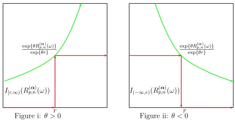
(1) is first established by Cramer. The RHS of (1) is also known as Chernoff’s bound. [See Dembo and Zeitouni(1999, page 26).] The intuition of (1) is that the upper bound can be made as close as possible to the upper tail of the return distribution by increasing the number of assets (n). The duality between P{R(α)
p,n(ω)> r} and P{R( α)
p,n(ω)< r} can be seen in Figures i and ii. Figure i shows that 1[r,∞)'R(α)
p,n(ω)( ≤ exp{θR (α) p,n(ω)}
exp{θr} if θ >0. Therefore, the upper tail
proba-bility can be written as
P{R(α)
p,n(ω)> r} )
=E[1[r,∞)(R(α) p,n(ω))]
*
≤ E+exp{θR
(α) p,n(ω)} exp{θr}
,
= exp-−'θr−logE[exp{θR(α) p,n(ω)}]
(.
= exp{−Λn(r,θ,α)}, (2)
where Λn(r,θ,α) = θr−logE[exp{θR(
α) p,n(ω)}].
function Λ(r,θ,α) w.r.t. θ and α, then sending (n) to infinity.
Similarly, Figure ii shows that the lower tail probability is
P{R(α)
p,n(ω)< r} )
=E[1(∞,r](R(α) p,n(ω))]
*
≤ E+exp{θR
(α) p,n(ω)} exp{θr}
,
= exp{−Λn(r,θ,α)}, (3)
where θ<0.
The RHS of (3) can be made as close as possible to the LHS by maximizing Λn(r,θ,α) w.r.t.
θ and α.
exp{θR(α) p,n(ω)} exp{θr}
r I[r,∞)(R(
α) p,n(ω))
Figure i: θ>0
exp{θR(α) p,n(ω)}
exp{θr}
r I(−∞,r)(R(
[image:7.595.93.477.292.493.2]α) p,n(ω))
Figure ii: θ<0
Furthermore, maximization of the RHS of (3) can be interpreted as the maximization of the expected value of the exponential utility function
U(R(α)
p,n(ω)) =− /
exp{R(α) p,n(ω)} exp{r}
0θ
,
which has the first and second derivatives
U!(R(α)
p,n(ω)) = −θ /
exp{R(α) p,n(ω)} exp{r}
0θ
,
U”(R(α)
p,n(ω)) = −θ2 /
exp{R(α) p,n(ω)} exp{r}
0θ
Hence, the Arrow-Pratt measure of absolute risk aversion is defined as
θAP =−
U”(R(α) p,n(ω))
U!
(R(α) p,n(ω))
=−θ.
In particular, when ˜ri, with i= 1, ..n are IID, Theorem 1 states that the RHS of (1) or (3) can be made as small as possible so that it can adequately approximate the LHS as (n) is sufficiently large.
Theorem 1. Let r+ = arg limn−→∞sup
1!α=1Λn(r,α) = ∞. Then, for r ∈ (E[˜r1], r
+) and a given α s.t. 1
!
α= 1 we have
P{R(α)
p,n(ω)> r}%
1 1
2π"n1α2
iθ(r)σ(r)
exp{−Λn(r,α)},
where R(α)
p,n(ω) is defined in (1), Λn(r,α) = sup
θ>0
-rθ −logE[exp{θR(α) p,n(ω)}]
.
with θ(r) = arg supθ>0-rθ−logE[exp{θR(α)
p,n(ω)}] .
and σ2(r) = 1
θ!
(r). Similarly, let r− = arg limn−→∞inf1!
α=1Λn(r,α) =∞. Then, for r∈(r
−, E[˜r
1]) we have
P{R(α)
p,n(ω)< r}%
1 1
2π"n1α2
iθ(r)σ(r)
exp{−Λn(r,α)},
whereΛn(r,α) = sup
θ<0
-rθ−logE[exp{θR(α) p,n(ω)}]
.
withθ(r) = arg supθ<0-rθ−logE[exp{θR(α) p,n(ω)}]
.
and σ2(r) = 1
θ!
(r).
Proof. See Appendix.
As shown in Remark 4.1 of Appendix A, in order to ensure that the deviations function for the lower tail probability/the upper tail probability has a unique maximal value, the benchmark (r) in Theorem 1 must be set below/above the mean valueE[R(α)
p,n(ω)].
function (mgf), i.e.,
E[exp{θR(α)
p,n(ω)}] = exp #
θ(αE[˜r1] + (1−α)E[˜r2]) +
θ2 2
)
α2V ar[˜r1] + (1−α)2V ar[˜r2] + 2α(1−α)Cov[˜r1,r˜2]
*
+ remainder&. (4)
In (4), the positions of θ and α can be exchanged without essentially changing the value of the deviations function as long as we have a finite truncation.
Therefore, maximization of the expected exponential utility (or the deviations function) is equivalent to minimization of the upper bound of the underperformance probability. That is
min 0<α<1P{R
(α)
p,n(ω)< r} ! − max
θ<0 0<α<1
−E+exp{R
(α) p,n(ω)} exp{r}
,θ
= min
θ<0 0<α<1
exp{−Λ2(r,θ,α)} = exp-− max
θ<0 0<α<1
Λ2(r,θ,α).. (5)
Since the number of risky assets are small the RHS of (5), that is defined as the risk bound, may not be close enough to the LHS. Hence, the optimal portfolio (ˆα) found in (5) can be interpreted as the value that maximizes the expected exponential utility and minimizes the risk bound simultaneously.
Remark 2.1. By the large deviations principle in (Dembo and Zeitouni, 1999), the benchmark
(r) in (5) must be set below E[R(α)
p,n(ω)] to ensure that a unique maximal value of the deviations function exist. Since E[R(α)
p,n(ω)] is the population mean that depends on a unknown quantity (α), the benchmark can empirically be set below the sample mean of a typical asset. Moreover, regarding the upper tail of the return distribution as in (2), (r) must be set above E[R(α)
p,n(ω)] for the existence of a unique maximal value.
Remark 2.2. As noted in (3), P rob{R(α)
p,n(ω) < r} can be approximated by maximizing the deviations function w.r.t. α and θ. Stutzer (2004) advocates that the risk-aversion parameter
para-meter can be assumed to depend on a set of feasible investments. The mathematical logic behind this idea is owed to the Gartner-Ellis theorem (see e.g. Dembo and Zeitouni, 1999, page 45) that applies the Fenchel Legendre transformation to show that the RHS of (3) converges to the LHS when (n) becomes large. However, by using asymmetry in the probability distribution of R(α)
p,n(ω), we can show a similar large deviations theorem without relying on the Fenchel Legendre transfor-mation. Whereby, the conventional utility approach can be maintained; i.e., an expected utility function should be only partially maximized. In another word, the expected utility function can be maximized w.r.t. (α) for any appropriately chosen risk-aversion parameter. Consequently, the
risk bound in (5) is dependent on the risk aversion parameter (θ). This point is clarified in next sections.
2.2
Implication of Asymmetry on Optimal Asset Allocation
Recent studies in the empirical finance literature have reported many evidences of two types of asymmetry in equity returns. [See e.g. (Patton,2004) and references therein.] The first is asym-metry in asset return distributions that leads to asymasym-metry in the portfolio return distribution, and the second is asymmetric dependence between two or more assets; i.e., asset returns appear to be more highly correlated during market downturns than during market upturns.
Now we provide a simple example just to illustrate the role played by asymmetric dependence and skewness in optimal investment problem. First, Let us define the first and second nonlinear correlations between two asset returns ˜r1 and ˜r2 as
λ12 =
E$[˜r1−E(˜r1)][˜r2−E(˜r2)]2 % 1
E[˜r1−E(˜r1)]2E[˜r2−E(˜r2)]4
,
λ21 =
E$[˜r1−E(˜r1)]2[˜r2−E(˜r2)] % 1
E[˜r1−E(˜r1)]4E[˜r2−E(˜r2)]2
.
skewness and probably lower variance. Moreover, let us define the skewness as
skew3(α) =
µ3(α)
µ3/22 (α),
where
µ3(α) = E[αr˜1+ (1−α)˜r2]3
= α3E[˜r13] + (1−α)3E[˜r32] + 3α2(1−α)E[˜r21r˜2] + 3α(1−α)2E[˜r1r˜22],
µ2(α) = E[αr˜1+ (1−α)˜r2]2
= α2E[˜r12] + (1−α)2E[˜r22] + 2α(1−α)E[˜r1˜r2].
Suppose thatE[˜r3
1] =E[˜r32] =−1,E[˜r12] =E[˜r22] = 1 andE[˜r1˜r2] = 0 we can compare investment strategies in two different cases as follows
1. Two assets are non-correlated, i.e. E[˜r21r˜2] =E[˜r1r˜22] = 0, we shall examine two strategies
(a) α= 0.5: skew3(0.5) =−0.714, µ2(0.5) = 0.5 (b) α= 0.4: skew3(0.4) =−0.756, µ2(0.4) = 0.52.
Since Strategy (a) has a lower variance and a higher skewness, thus Strategy (a) is obviously preferred to Strategy (b).
2. Two assets are non-linearly correlated, i.e. E[˜r2
1˜r2] = −0.3 and E[˜r1r˜22] = 0.9, we shall examine two strategies
(a) α= 0.5: skew3(0.5) =−0.071, µ2(0.5) = 0.5 (b) α= 0.4: skew3(0.4) = 0.06, µ2(0.4) = 0.52.
Hence, it is interesting to examine the implication of asymmetry in a portfolio return distribution and asymmetric dependence on optimal asset allocation. First, a parametric model is proposed to capture the asymmetric characteristics of portfolio return distribution. Next, an Edgeworth expansion can be applied to pick out the nonlinear correlations of asset returns (λ12, λ21), whereby we can examine their effects on an optimal portfolio choice and its risk bound.
2.3
Parametric Implementation
2.3.1 Large portfolio optimization technique
The deviations function in (5) is the Fenchel-Legendre transformation of the logarithm of the mgf. If individual returns are uncorrelated, the mgf of the portfolio return is simply the product of the individual mgfs, thus no assumption on the portfolio return distribution is necessary. A standard optimization technique can then be applied to maximize the deviations function. However, when individual returns are not uncorrelated, it is necessary to impose an explicit assumption on the portfolio return distribution. This portfolio optimization technique is based on 1) maximizing the expected log likelihood function of the portfolio return 2) maximizing the deviations function in (5) w.r.t. the investment proportion (α) for a given degree of absolute risk aversion. Note that the degree of absolute risk aversion should be chosen in the vicinity of the maximal values (θ∗,α∗) of the deviations function so that the RHS of (5) can be tightened to the LHS by an
asymptotic argument.
In another word, maximization of an expected log likelihood function, that is interpreted as the minus of the empirical entropy of the portfolio return, is equivalent to minimization of the uncertainty level of the portfolio return. Moreover, as shown in (3), maximization of a deviations function is equivalent to maximization of an expected utility function. Both can be associated with minimization of the risk that the portfolio return may fall below an investable benchmark.
Suppose that there are (n) risky assets, the portfolio return is given by
R(α)
p,n(ω) = n−1 2
i=1
αir˜i+ (1− n−1 2
i=1
αi)˜rn
= α
!
where α
!
={α1, ..,αn−1} and ˜r
!
={r˜1, ..,r˜n−1}.
Let us assume that R(α)
p,n(ω) ∼ pdf '
R(α) p,n(ω)|Θ
(
, where R(α)
p,n(ω) stresses that Rp depends on (α) and (n). Given a sample of size T {˜rt}T
t=1, the log-likelihood function can be written as
'(Θ,α) = 1
T
T 2
t=1
logpdf'R(α)
p,n,t(ω)|Θ (
.
Therefore, the ML estimate of Θ is
3
Θ(α) = arg max Θ∈A'(Θ,
α) (6)
for a given α, whereA is a compact set containing the true parameters, and Θ3(α) stresses that the ML estimate depends on a specific α. The ideal case is when Θ3(α) is a function of α. Otherwise, we can rely on an interpolation technique to find an approximation of Θ3(α) that is a polynomial of (α).
Furthermore, in view of (5) it can be shown that as the number of risky assets (n) is large, we have
logP{R(α)
p,n(ω)< r} ≈− max
θ<0 α∈S
$
rθ−log exp{θR(α) p,n(ω)}
%
= −max
θ<0 α∈S
Λn)r,θ,Θ3(α)
*
,
whereS is the set of feasible investments. (The formal result for asymmetric return distributions will be given in the next section.)
For a given risk-aversion parameter (ˆθ < 0) in the vicinity of (θ∗) that is obtained by total
maximization of Λn)r,θ,Θ3(α)
*
, the optimal portfolio is given as
ˆ
α(ˆθ) = arg max
α∈S
⇔
ˆ
α(ˆθ) = arg
#
α: ∂Λ(r,
ˆ
θ,Θ)
∂Θ 4 4 4
Θ=Θ(α)
∂Θ3(α)
∂α = 0
&
. (7)
Suppose that the distributions of ˜r are pdf(˜ri) with the central moments µi,m =E$r˜i−E[˜ri]%m
for i= 1, .., n, then we have the following relationship
E$R( ˆα)
p,n(ω)−E[R( ˆ α) p,n(ω)]
%m
= E$
n 2
i=1
(˜ri−µi,1) %m = E / n 2 i=1 i k=1mk=m 5 m m1, ..., mi
67j=i
j=1
[ˆαj(˜rj −µj,1)]mj 0 = n 2 i=1 ˆ
αmi E$r˜i−E[˜ri] %m + n 2 i=2 i k=1mk=m mi&=m, ∀ i=2,..,n
5
m m1, .., mi
67i
j=1 ˆ
αmjj E$
i 7
j=1
[˜rj −µj,1]mj % = n 2 i=1 ˆ
αmi µi,m+
n 2
i=2 i
k=1mk=m mi&=m,∀ i=2,..,n
5
m m1, .., mi
67i
j=1 ˆ
αmjj ρm1,..mi, (8)
where ρm1,..mi ∀ i= 2, .., n are the measures of covariance.
Hence, for an optimal portfolio as given in (7), the individual central moments, and the central moments of the pdf of Rαˆ
p,n(ω) that is estimated by (6), the relationship among the measures of correlation that is denoted by the second term in the RHS of (8) can be recovered by using (8). Although this technique does not enable us to effectively recover the individual values of the high order measures of correlation, an interesting implication of (8) is that although the individual nonlinear correlations may not effect the optimal portfolio and the risk, an appropriate linear combination of the individual linear correlation or the nonlinear ones, that contributes to a decrease in the portfolio variance or an increase in the portfolio skewness, can have a strong impact on the optimal portfolio and the risk. We will address this further in the empirical analysis.
portfolio returnR(α)
p,n(ω) can be straightforwardly derived from the distributions of the individual returns. For instance, the weighted sums of Normal, Gamma, or Chi squared random variables are Normal, Gamma, or Chi squared distributed respectively. (See Rao, 1973 for the proofs.) However, when asset returns are dependent, it is rather complicated to derive the distribution of the portfolio return that is usually dependent on a specific assumption about dependence. Thus, in this section we assume a certain parametric form for the portfolio return distribution that depends on an investable portfolio (α). As a consequence, the measures of covariance can be recovered from the relationship (8), thus explicitly depend on the optimal portfolio ( ˆα). An explanation is that the probabilities of the extreme values of R(α)
p,n(ω) are so small that they contribute negligibly to the value of the average log-likelihood function (6). Thus, it is sensible to choose a proportion ( ˆα) such that the frequency of realizations of R(
α)
p,n(ω) in the lower tail of the portfolio return distribution is as small as possible. This is consequently equivalent to selecting a portfolio ( ˆα) such that the underperformance probability is minimized whilst the expected utility function is maximized. This idea can be summarized in the following remark.
Remark 2.3. The optimal portfolio (αˆ) is the maximal value of the deviations function and the
minimal value of the frequency of the lower tail extreme values of R(α)
p,n(ω). Thus, the recovered measures of covariance are dependent on αˆ.
In order to illustrate how this technique works, let us assume that there are two risky assets; and that the portfolio return is normal distributed, i.e.,
pdf'R(p,2α)(ω)( = √ 1 2πσp
exp 8
− 12 9R(α)
p,2(ω)−µp
σp
:2;
,
mgf(θ) = exp-θµp+
θ2 2σ
2 p .
Then, the ML estimates of µp and σp are
ˆ
µp(α) = 1
T
T 2
t=1
Rp,2(α)(ω),
ˆ
σ2p(α) = 1
T
T 2
t=1
(R(p,2α)(ω)−µˆp(α))2,
∂µˆp(α)
∂α = 1 T T 2 t=1
(˜r1t−r˜2t),
∂σˆp2(α)
∂α = 2 T T 2 t=1 '
R(p,2α)(ω)−µˆp(α) (
(˜r1,t−˜r2,t).
Let θ∗ denotes the maximal value obtained by maximizing Λn(r,θ,α) w.r.t. α and θ. Then, for a given ˆθ in the neighbourhood of θ∗ αˆ(ˆθ) is a solution to
ˆ
θ∂µˆ(α) ∂α +
ˆ
θ2 2
∂σˆ2(α)
∂α = 0.
Hence, we have
ˆ
α(ˆθ) = −A
B,
where A and B are defined as
A = ˆθ#1
T(2−
1
T)[
T 2
t=1
(˜r1t−˜r2t)]2− T 2
t=1
(˜r1t−r˜2t)2 &
− T 2
t=1
(˜r1t−r˜2t),
B = ˆθ#
T 2
t=1 ˜
r2t(˜r1t−r˜2t)−
T2−T −1
T T 2 t=1 ˜ r2t T 2 t=1
(˜r1t−r˜2t) &
.
2.3.2 Asymmetric Gamma distribution
asset returns. In view ofKnight et al.(1995), our analysis is based on two cases; 1) asset returns are uncorrelated, and 2) asset returns are correlated. First, we state the statistical properties of the asymmetric Gamma distribution and the (partially) symmetric Gamma distribution.
1. The Asymmetric Gamma Distribution
A return distribution is a mixture of two Gamma distributions, i.e.,
˜
r∼mixture'p,Gamma(γ1,κ1),Gamma(γ2,κ2) (
if its values depend on whether return is positive or negative. The probability density is given by
pdf(˜r) =pI[0,∞)(˜r) 1
γκ1 1 Γ(κ1)
˜
rκ1−1exp{− r˜
γ1}
+ (1−p)I(−∞,0)(˜r) 1
γκ2 2 Γ(κ2)
(−r˜)κ2−1exp{r˜
γ2}
,
where γ1 and γ2 are positive. Γ(•) is the standard Gamma function. Given a sample of sizeT {r˜t}Tt=1, the likelihood function can be written as
T 7
t=1
pdf(˜rt) = T 7
t=1 #
pI[0,∞)(˜rt) 1
γκ1 1 Γ(κ1)
˜
rκ1−1
t exp{− ˜
rt
γ1}
+ (1−p)I(−∞,0)(˜rt) 1
γκ2 2 Γ(κ2)
(−r˜t)κ2−1exp{ ˜
rt
γ2} &
. (9)
Since the RHS of (9) is the product of sums of the orthogonal terms, we have
T 7
t=1
pdf(˜rt) = p#{t∈[1,T]: ˜rt≥0}(1−p)T−#{t∈[1,T]: ˜rt≥0}
7
t∈{t∈[1,T]: ˜rt≥0}
#
I[0,∞)(˜rt) 1
γκ1 1 Γ(κ1) ˜
rκ1−1
t exp{− ˜
rt
γ1}
& 7
t∈{t∈[1,T]: ˜rt<0}
#
I(−∞,0)(˜rt) 1
γκ2 2 Γ(κ2)
(−r˜t)κ2−1exp{ ˜
rt
γ2} &
,
where #{t ∈ [1, T] : ˜rt ≥ 0} is the number of the nonnegative return realizations in the sample.
likeli-hood function can be written as
'(γ1,γ2,κ1,κ2) = #{t ∈[1, T] : ˜rt≥0}log(ˆp) + (T −#{t∈[1, T] : ˜rt>0}) log(1−pˆ) + (κ1−1)
2
t∈{t∈[1,T]: ˜rt≥0}
log(˜rtI[0,∞)(˜rt))− 1
γ1
2
t∈{t∈[1,T]: ˜rt≥0}
˜
rtI[0,∞)(˜rt)
− #{t ∈[1, T] : ˜rt≥0} )
κ1log(γ1) + log(Γ(κ1)) *
+ (κ2−1)
2
t∈{t∈[1,T]: ˜rt<0}
log'−r˜tI(−∞,0)(˜rt) (
+ 1
γ2
2
t∈{t∈[1,T]: ˜rt<0}
˜
rtI(−∞,0)(˜rt)
− #{t ∈[1, T] : ˜rt<0} )
κ2log(γ2) + log(Γ(κ2)) *
.
By taking derivatives of'(γ1,γ2,κ1,κ2) w.r.t. (γ1,γ2,κ1,κ2), the ML estimates ( ˆγ1,γˆ2,κˆ1,κˆ2) are the solutions to
Γ!(κ1)
Γ(κ1) − log(κ1) = T
t=1log(˜rtI[0,∞)(˜rt))
#{t∈[1,T]: ˜rt≥0} −log
' "T t=1
˜
rtI[0,∞)(˜rt)
#{t∈[1,T]: ˜rt≥0}
(
,
Γ!(κ2)
Γ(κ2) − log(κ2) = T t=1log
'
−rtI˜ (−∞,0)(˜rt) (
#{t∈[1,T]: ˜rt<0} −log
'
− Tt=1˜rtI(−∞,0)(˜rt)
#{t∈[1,T]: ˜rt<0}
(
,
γ1 = T
t=1rtI˜ [0,∞)(˜rt) #{t∈[1,T]: ˜rt≥0}κ1,
γ2 = − T
t=1rtI˜ (−∞,0)(˜rt) #{t∈[1,T]: ˜rt<0}κ2.
(10)
Figure2 shows that the functions f(κ) = the LHS−the RHS of the first two equations in (10) are increasing, thus the ML estimates are the unique solutions to (10).
The asymptotic variances of ( ˆγ1,γˆ2,κˆ1,κˆ2) are the diagonal elements of the inverse of the sample information matrix as given by
I=T inv
Pκ∗2 1 P
∗
κ1γ1 P
∗
κ1γ2 P
∗
κ1,κ2
P∗
γ1κ1 P
∗
γ2 1 P
∗
γ1γ2 P
∗
γ1κ2
P∗
γ2κ1 P
∗
γ2γ1 P
∗
γ2 2 P
∗
γ2κ2
Pκ∗2κ1 Pκ∗2γ1 Pκ∗2γ2 Pκ∗2 2
(γ1,γ2,κ1,κ2)=( ˆγ1,γˆ2,κˆ1,κˆ2)
where
Pγ∗2
1 = #{t∈[1, T] : ˜rt≥0}
κ1
γ12 −
2
γ13
T 2
t=1 ˜
rtI[0,∞)(˜rt),
Pγ∗2
2 = #{t∈[1, T] : ˜rt<0}
κ2
γ22 +
2
γ23
T 2
t=1 ˜
rtI(−∞,0)(˜rt),
Pκ∗2
1 = −#{t∈[1, T] : ˜rt≥0} Γ”(κ
1)Γ(κ1)−(Γ
!
(κ1)2) Γ2(κ
1)
,
Pκ∗2
2 = −#{t∈[1, T] : ˜rt<0} Γ”(κ
2)Γ(κ2)−(Γ
!
(κ2)2) Γ2(κ
2)
,
Pγ∗1κ1 = −#{t∈[1, T] : ˜rt≥0} 1
γ1
,
Pγ∗2κ1 = −#{t∈[1, T] : ˜rt≥0} 1
γ2
,
Pγ∗1κ2 = Pγ∗1γ2)=Pκ∗1γ2 = 0*
where Γ!
and Γ” are the first and the second derivatives of the standard Gamma function.
2. The (Partially) Symmetric Gamma Distribution (i.e. γ1 =γ2)
Let us assume that the scale parameters (γ1, γ2) are equal. Thus, in this case the mo-ments become more symmetric than the other case. The case of complete asymmetry (i.e., both the scale parameters and the magnitude ones are the same) can be derived straightfor-wardly. Therefore, by applying the conventional MLE method, the ML estimates (ˆγ,κˆˆ1,κˆˆ2) for the partially symmetric Gamma distribution are the solutions to
Γ!(κ1) Γ(κ1) −log
)
#{t∈[1, T] : ˜rt≥0}κ1+ #{t∈[1, T] : ˜rt<0}κ2 *
= 1
#{t∈[1,T]: ˜rt≥0}
"T
t=1log(˜rtI[0,∞)(˜rt))−log"Tt=1r˜t '
I(0,∞)(˜rt)−I(−∞,0)(˜rt) (
,
Γ!(κ2) Γ(κ2) −log
)
#{t∈[1, T] : ˜rt≥0}κ1+ #{t∈[1, T] : ˜rt<0}κ2 *
= #{t∈[1,T1]: ˜rt<0}"Tt=1log(−r˜tI(−∞,0)(˜rt))−log"Tt=1˜rt '
I(0,∞)(˜rt)−I(−∞,0)(˜rt) (
,
γ =
T t=1˜rt
'
I(0,∞)(˜rt)−I(−∞,0)(˜rt)
(
#{t∈[1,T]: ˜rt≥0}κ1+#{t∈[1,T]: ˜rt<0}κ2.
information matrix as given by
I=T inv
Pκ∗2 1 P
∗
κ1γ P
∗
κ1,κ2
Pγκ∗ 1 Pγ∗2 Pγκ∗ 2
P∗
κ2κ1 P
∗
κ2γ P
∗
κ2 2
(γ,κ1,κ2)=(ˆγ,κˆˆ1,κˆˆ2)
,
where
Pγ∗2 = − 2
γ3 T 2
t=1 ˜
rt '
I(0,∞)(˜rt)−I(−∞,0)(˜rt) (
+ #{t∈[1, T] : ˜rt≥0}
κ1
γ2,
Pγκ∗ 1 = −#{t∈[1, T] : ˜rt≥0} 1
γ,
Pγκ∗ 2 = −#{t∈[1, T] : ˜rt<0} 1
γ,
Pκ∗2
1 = −#{t∈[1, T] : ˜rt≥0}
Γ”(κ1)Γ(κ1)−(Γ
!
(κ1))2 Γ2(κ
1)
,
Pκ∗2
2 = −#{t∈[1, T] : ˜rt<0} Γ”(κ
2)Γ(κ2)−(Γ
!
(κ2))2 Γ2(κ
2)
,
Pκ∗1κ2 = 0.
The likelihood ratio (LR) test for the null hypothesis of partial asymmetry against the alternative one of symmetry (i.e., γ1 =γ2) can be formulated as
LR= 2)'(ˆγ1,γˆ2,κˆ1,κˆ2)−'(ˆγ,κˆˆ1,κˆˆ2) *
∼χ2(1), (11)
where χ2(1) is the Chi squared distribution with 1 degree of freedom. Next, let us assume that the portfolio return (R(α)
aver-sion parameter is required to remain in the neighbourhood of the totally maximal value of the deviations function.
Theorem 2. Suppose that the return of a portfolio of (n) risky assets
R(α)
p,n(ω) =α
!
˜
r+ (1−1!α)˜rn,
where α
!
= (α1, ..,αn−1) and ˜r
!
= (˜r1, ..,r˜n−1), is asymmetrically distributed, we have
lim n−→∞
1
nsupα∈S
log)P'R(α)
p,n(ω)> r (*
=−#θˆr− lim n−→∞
1
nsupα∈S +
logE
P'R(α) p,n(ω)
($exp-nθˆR(α) p,n(ω)
.%,&
,
(12) where S is a compact set of feasible investments, θˆis in the neighbourhood ofθ∗, andP'R(α)
p,n(ω)( is the portfolio return distribution. Furthermore,
θ∗ = arg lim n−→∞
1
nαinf∈S sup
θ∈(0,∞) #
nθr−logE
P'R(α)
p,n(ω)($exp
-nθR(α) p,n(ω)
.%&
.
Similarly, we have
lim n−→∞
1
nαinf∈S
log)P'R(α)
p,n(ω)< r (*
=−#θˆr+ lim n−→∞
1
nsupα∈S +
−logE
P'R(α) p,n(ω)
($exp-nθˆR(α) p,n(ω)
.%,&
,
(13) where θˆis in the neighbourhood ofθ∗, where
θ∗ = arg lim n−→∞
1
nθ∈sup(−∞,0) α∈S
#
nθr−logE
P'R(α) p,n(ω)
($exp-nθR(α) p,n(ω)
.%&
.
Proof. See Appendix.
or (13) is a monotonic function, the solution is trivial since the optimal portfolio lies on the boundary of the investment set S.
As shown in Section 2.3.1, when a portfolio is very large, the number of individual central moments increases; the structure of dependence becomes rather complicated. This can hinder our analysis of the effects of individual skewnesses and correlations on optimal portfolio and asymmetric risk. For ease of exposition, we analyze the case when there are two risky assets. First, the case of two independent asset returns is analyzed.
2.3.3 Assets are uncorrelated
The mgf ofR(p,2α)(ω) =α˜r1+(1−α)˜r2, where ˜ri ∼ mixture '
pi,Gamma(γi,1,κi,1),Gamma(γi,2,κi,2) (
for i= 1,2 as defined in Section 2.3.2, is given by
mgf(θ,α) = p1p2
1
(1−θαγ1,1)κ1,1(1−θ(1−α)γ2,1)κ2,1 + (1−p1)(1−p2)
1
(1 +θαγ1,2)κ1,2(1 +θ(1−α)γ2,2)κ2,2 + p1(1−p2)
1
(1−θαγ1,1)κ1,1(1 +θ(1−α)γ2,2)κ2,2 + p2(1−p1)
1
(1 +θαγ2,1)κ2,1(1−θ(1−α)γ1,2)κ1,2
, (14)
where the parameters (γi,1,κi,1,γi,2,κi,2) fori= 1,2 can be estimated from actual data by using the procedures described in Section 2.3.2.
To study the effects of the individual skewnesses or all the other high order moments of
moment) is given by
E2(θ,α) = exp #
θE[R(p,2α)(ω)] + 1 2θ
2E$R(α)
p,2(ω)−E[R (α) p,2(ω)]
%2
+ remainder&
= exp#θ)α(p1γ1,1κ1,1−(1−p1)γ1,2κ1,2) + (1−α)(p2γ2,1κ2,1−(1−p2)γ2,2κ2,2) *
+ 1
2θ 2)α(p
1γ1,12 κ1,1+ (1−p2)γ2,22 κ2,2) + (1−α)(p2γ2,12 κ2,1+ (1−p2)γ2,22 κ2,2) *
+ remainder&. (15)
The third order Edgeworth expansion (i.e., the mgf is truncated up to the third moment) is given by
E3(θ,α) = exp #
θE[R(p,2α)(ω)] + 1 2θ
2E$R(α)
p,2(ω)−E[R (α) p,2(ω)]
%2 +1
6θ
3E$R(α)
p,2(ω)−E[R (α) p,2(ω)]
%3
+ remainder&
= exp#θ)α(p1γ1,1κ1,1−(1−p1)γ1,2κ1,2) + (1−α)(p2γ2,1κ2,1−(1−p2)γ2,2κ2,2) *
+ 1
2θ 2)α(p
1γ1,12 κ1,1+ (1−p2)γ2,22 κ2,2) + (1−α)(p2γ2,12 κ2,1+ (1−p2)γ2,22 κ2,2) *
+ 1
3θ 3)α(p
1γ1,13 κ1,1−(1−p2)γ2,23 κ2,2) + (1−α)(p2γ2,13 κ2,1−(1−p2)γ2,23 κ2,2) *
+ remainder&. (16)
As justified in (3), the underperformance probability is always bounded from above by exp{−Λ2(r,θ,α)}, where Λ2(r,θ,α) =rθ−log'mgf(θ,α)(. (mgf(θ,α) and its approximations are given in (14),
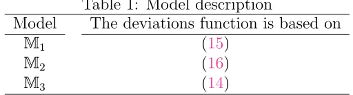
(15), and (16) respectively.) Thus the upper bound is called the risk bound. To find an optimal portfolios for a given risk-aversion degree ˆθ, we can use the Newton Raphson Algorithm to max-imize −mgf(ˆθ,α), E2(ˆθ,α), andE3(ˆθ,α) respectively2. Now, let us specify the following models:
Model M1 in Table 1 is used as a benchmark for the other models. In order to test whether there is an effect of individual skewnesses or other high order moments on the optimal portfolio and the risk bound, we need to formulate a set of statistical hypotheses as follows:
2
As shown in Burden and Fairs (1997), this algorithm has the degree of convergence N1/2
, where (N) is the
Table 1: Model description
Model The deviations function is based on
M1 (15)
M2 (16)
M3 (14)
1. The null hypothesis that there is a sole effect of the skewnesses on the optimal portfolio is
H(1)
0 : |αˆM2θˆ)−αˆM1(ˆθ)|≤-, (17)
where - is an arbitrary small positive number, and ˆθ is a given risk aversion parameter.
2. The null hypothesis that there are effects of the skewnesses and all the other high order moments on the optimal portfolio is
H(2)
0 : |αˆM3(ˆθ)−αˆM1(ˆθ)|≤-. (18)
To test the null hypotheses H(1)
0 and H (2)
0 , The one-cell contingency table test can be used. [See Rao (1973, page 393).] First, let us denote (N) samples of the same size (T) drawn from the true return distributions as #-(˜r1t(i),˜r2t(i)).Tt=1&N
i=1. However, we can split up a big sample of data in to (N) small subsamples. Then, the t test for the hypothesis H(1)0 is given by
t= o1−e1
e1
+ o2−e2
e2 ∼
χ2(1), (19)
where
o1 = #{i∈[1, N] : |αˆM2,i(ˆθ)−αˆM1,i(ˆθ)|≤-},
o2 = N −o1,
e1 = 0.95N,
where ˆαM2,i(ˆθ) fori= 1, .., N are the optimal portfolios estimated from the subsamples.
The ttest for the hypothesisH(2)0 can also be formulated in a similar way. Furthermore, since skewness and asymmetry are typical features of asset returns, we believe that they have a strong effect on optimal portfolio, thus risk bound. This logic implies that the test for a sole effect of skewnesses on the optimal portfolio is equivalent to the test for asymmetry in the portfolio return distribution.
2.3.4 Assets are correlated
When asset returns are pairwise correlated, in view of Theorem2we need to specify a distribution for the portfolio return so that the mgf can be evaluated. An appropriate candidate is the asymmetric Gamma distribution as defined in Section 2.3.2. We apply the general theory given in Section 2.3.1 to construct parametrically optimal portfolios from actual return data.
Following Section 2.3.3, assuming that there are two risky assets. The portfolio return is
Rp,2(α)(ω) =α˜r1+(1−α)˜r2, whereR(p,2α)(ω)∼ mixture )
p(α),Gamma(γ1(α),κ1(α)),Gamma(γ2(α),κ2(α)) *
. Then, we have two different cases.
• The Asymmetric Portfolio Return Distribution
ˆ
γ2(α),κˆ2(α),pˆ(α) *
, which are the functions of α, are the solutions to (20)-(24), i.e.,
Γ!(κ1(α)) Γ(κ1(α)) −
log'κ1(α) (
= "T
t=1log '
R(p,2,tα) (ω)I[0,∞)(R(p,2,tα) (ω)) (
#{t∈[1, T] : Rp,2,t(α) (ω)≥0} − log
5"T t=1R
(α)
p,2,t(ω)I[0,∞)(R(p,2,tα) (ω)) #{t ∈[1, T] : Rp,2,t(α) (ω)≥0}
6
, (20)
Γ!
(κ2(α)) Γ(κ2(α)) −
log'κ2(α) (
= "T
t=1log '
−R(p,2,tα) (ω)I(−∞,0)(R(p,2,tα) (ω)) (
#{t ∈[1, T] : Rp,2,t(α) (ω)<0} − log
5 −
"T t=1R
(α)
p,2,t(ω)I(−∞,0)(R(p,2,tα) (ω)) #{t ∈[1, T] : Rp,2,t(α) (ω)<0}
6
, (21)
γ1(α) =
"T t=1R
(α)
p,2,t(ω)I[0,∞)(R(p,2,tα) (ω)) #{t∈[1, T] : Rp,2,t(α) (ω)≥0}κ1(α)
, (22)
γ2(α) = − "T
t=1R (α)
p,2,t(ω)I(−∞,0)(Rp,2,t(α) (ω)) #{t∈[1, T] : Rp,2,t(α) (ω)<0}κ2(α)
, (23)
p(α) = #{t∈[1, T] : R (α)
p,2,t(ω)≥0}
T . (24)
• Partially Symmetric Portfolio Return Distribution
' ˆ
γ(α),κˆ1(α),κˆ2(α),pˆ(α) (
are the solutions to (25)-(28), i.e.,
Γ!(κ1(α)) Γ(κ1(α)) −
log)#{t∈[1, T] : Rp,2,t(α) (ω)≥0}κ1(α) + #{t∈[1, T] : Rp,2,t(α) (ω)<0}κ2(α) *
= 1
#{t ∈[1, T] : Rp,2,t(α) (ω)≥0} T 2
t=1
log)R(p,2,tα) (ω)I[0,∞)(Rp,2,t(α) (ω)) *
− log T 2
t=1
R(p,2,tα) (ω)'I[0,∞)(Rp,2,t(α) (ω))−I(−∞,0)(Rp,2,t(α) (ω)) (
, (25)
Γ!
(κ2(α)) Γ(κ2(α)) −
log)#{t∈[1, T] : Rp,2,t(α) (ω)≥0}κ1(α) + #{t∈[1, T] : Rp,2,t(α) (ω)<0}κ2(α) *
= 1
#{t ∈[1, T] : Rp,2,t(α) (ω)<0} T 2
t=1
log'−Rp,2,t(α) (ω)I(−∞,0)(R(p,2,tα) (ω)) (
− log T 2
t=1
R(p,2,tα) (ω)'I[0,∞)(Rp,2,t(α) (ω))−I(−∞,0)(Rp,2,t(α) (ω)) (
, (26)
γ(θ) =
"T t=1R
(α) p,2,t(ω)
'
I[0,∞)(Rp,2,t(α) (ω))−I(−∞,0)(R(p,2,tα) (ω)) (
#{t ∈[1, T] : Rp,2,t(α) (ω)≥0}κ1(α) + #{t ∈[1, T] : R(p,2,tα) (ω)<0}κ2(α)
, (27)
p(α) = #{t ∈[1, T] : R (α)
p,n,t(ω)≥0}
T . (28)
Note that neither (20)-(24) nor (25)-(28) exist close form solutions. For brevity, we shall focus on (20)-(24); (25)-(28) can be handled in a similar way. An interpolation technique can be applied to estimate )γˆ1(α),κˆ1(α),γˆ2(α),κˆ2(α),pˆ(α)
*
. Cubic splines (see e.g., Burden and Fairs, 1997) can be used to fit these relationships.
Let)cs1(α),cs2(α),cs3(α),cs4(α),cs5(α) *
denote the fitted cubic splines of the ML estimates )
ˆ
γ1(α),κˆ1(α),ˆγ2(α),κˆ2(α),pˆ(α) *
resp. Then, the fitted mgf of R(p,2α)(ω) is given by
F
mgf(θ,α) = cs5(α) 5
1 1−θcs1(α)
6cs2(α)
+'1−cs5(α)
(5 1
1 +θcs3(α) 6cs4(α)
. (29)
of the fitted mgf can be used. The second order Edgeworth expansion is given by
3
E2(θ,α) = exp 8
θ'cs5(α)cs1(α)cs2(α)−(1−cs5(α))cs3(α)cs4(α) (
+ 1
2θ 2'cs
5(α)cs21(α)cs2(α) + (1−cs5(α))cs23(α)cs4(α) (
+ remainder ;
. (30)
The third order Edgeworth expansion is given by
3
E3(θ,α) = exp 8
θ'cs5(α)cs1(α)cs2(α)−(1−cs5(α))cs3(α)cs4(α) (
+ 1
2θ 2'cs
5(α)cs21(α)cs2(α) + (1−cs5(α))cs23(α)cs4(α) (
+ 1
3θ 3'cs
5(α)cs31(α)cs2(α)−(1−cs5(α))cs33(α)cs4(α) (
+ remainder ;
. (31)
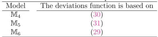
[image:28.595.174.429.460.521.2]As shown in Theorem 2, the optimal portfolios 'αˆ(ˆθ)( are the maximal values of −mgfF(ˆθ,α), −E32(ˆθ,α), and −E33(ˆθ,α) resp., where ˆθ is in the neighbourhood of θ∗ as defined in Theorem 2. The models are summarized in Table 2. For the (partially) symmetric case as defined by
Table 2: Model descriptions
Model The deviations function is based on
M4 (30)
M5 (31)
M6 (29)
(25)-(28), we can define the modelsM7 (the benchmark model),M8 (the third order Edgeworth expansion), and M9 (the exact moment) in a similar way.
As pointed out in (8), although high order measures of correlations can not be recovered from the central moments of the optimal portfolio return, their pairwise linear relationships can be recovered, i.e.,
ˆ
λ11 =
E$R( ˆp,2α)(ω)−E[R( ˆp,2α)(ω)]%2−αˆ2E$r˜1−E[˜r1] %2
−(1−αˆ)2E$r˜
2−E[˜r2] %2 G
E$r˜1−E[˜r1] %2
E$r˜2−E[˜r2]
ˆ
λ21αˆ2(1−αˆ) G
E$r˜1−E[˜r1] %4
E$r˜2−E[˜r2] %2
+ ˆλ12αˆ(1−αˆ)2 G
E$˜r1−E[˜r1] %2
E$r˜2−E[˜r2] %4
= 2
3√6 5
E$R( ˆp,2α)(ω)−E[R( ˆp,2α)(ω)]%3−αˆ3E$r˜1−E[˜r1] %3
−(1−αˆ)3E$r˜2−E[˜r2] %36
, (33)
where
E$R( ˆp,2α)(ω)−E[R( ˆp,2α)(ω)]%2 = cs5(ˆα)cs21(ˆα)cs2(ˆα) + (1−cs5(ˆα))cs23(ˆα)cs4(ˆα),
E$R( ˆp,2α)(ω)−E[R( ˆp,2α)(ω)]%3 = cs5(ˆα)cs31(ˆα)cs3(ˆα)−(1−cs5(ˆα))cs33(ˆα)cs4(ˆα),
E$r˜1−E[˜r1] %2
= ˆp1γˆ1,12 κˆ1,1+ (1−pˆ1)ˆγ1,22 κˆ1,2,
E$r˜1−E[˜r1] %3
= ˆp1γˆ1,13 κˆ1,1−(1−pˆ1)ˆγ1,23 ˆκ1,2,
E$r˜1−E[˜r1] %4
= ˆp1γˆ1,14 κˆ1,1+ (1−pˆ1)ˆγ1,24 κˆ1,2,
E$r˜2−E[˜r2] %2
= ˆp2γˆ2,12 κˆ2,1+ (1−pˆ2)ˆγ2,22 κˆ2,2,
E$r˜2−E[˜r2] %3
= ˆp2γˆ2,13 κˆ2,1−(1−pˆ2)ˆγ2,23 ˆκ2,2,
E$r˜2−E[˜r2] %4
= ˆp2γˆ2,14 κˆ2,1+ (1−pˆ2)ˆγ2,24 κˆ2,2,
and ˆλ11is the recovered linear correlation. ˆλ12and ˆλ21are the recovered first nonlinear correlation and the recovered second one as given in Section2.2. ˆαis the optimal portfolio estimated from the models in Table 2. The other parameters with hats (3) are the ML estimates of the asymmetric Gamma distributions as defined in Section 2.3.2.
correlations such that the total impact of asymmetric dependence on the optimal portfolio is negligible. We will address this point further in Section 3.
Let M4 denotes the benchmark model. In order to test whether there is an effect of the second order nonlinear correlations or the other high order nonlinear correlations on the optimal portfolio, we need to formulate a set of statistical hypotheses as follows:
1. The null hypothesis that there is a sole effect of the second order nonlinear correlations on the optimal portfolio is
H(3)
0 : |αˆM5(ˆθ)−αˆM4(ˆθ)|≤-, (34) where-is an arbitrary small number. ˆθis in the neighbourhood ofθ∗ as defined in Theorem 2.
2. The null hypothesis that there is an effect of the other high order nonlinear correlations on the optimal portfolio is
H(4)
0 : |αˆM6(ˆθ)−αˆM4(ˆθ)|≤-, (35) where ˆαM4, ˆαM5, and ˆαM6 are the optimal portfolios estimated from the models in Table2.
The null hypotheses for the partially symmetric case (i.e., the modelsM7−M9) can be formulated similarly. The one-cell contingency table test as proposed in Section 2.3.3 can be used to test H(3)
0 and H (4)
0 . However, since asymmetric dependence is a typical phenomenon in the market, thus it has an evident impact on optimal asset allocation (see e.g. Patton,2004). We will confirm that there is a strong effect of the second order nonlinear correlations on the optimal portfolio by using some empirical evidences.
3
EMPIRICAL EVIDENCE
In this section, we provide some short simulations to illustrate the portfolio optimization tech-nique proposed in Section 2. By using equity data Bangkok SET index3 and S&P 500, we also investigate empirically the effect of individual skewnesses and nonlinear correlations on optimal
3
portfolio and risk bound.
1. Data description
Data of Bangkok SET and S&P 500 are available monthly from 1975 to 2001. Arithmetic return is calculated by ˜rt = Pt−Pt
−1
Pt−1 . The sample statistics of the returns are reported in Table 3. The kernel return densities are plotted in Figure1. The mean and the variance of S&P 500 are higher while the kurtosises are roughly equal. However, Bangkok SET has a positive skewness while S&P 500 has a negative one. The first sample nonlinear correlation and the second one, that are apparently unequal, indicate a strong asymmetric dependence between the two assets. Hence, in view of the example given in Section 2.2, this case is indeed interesting to investigate.
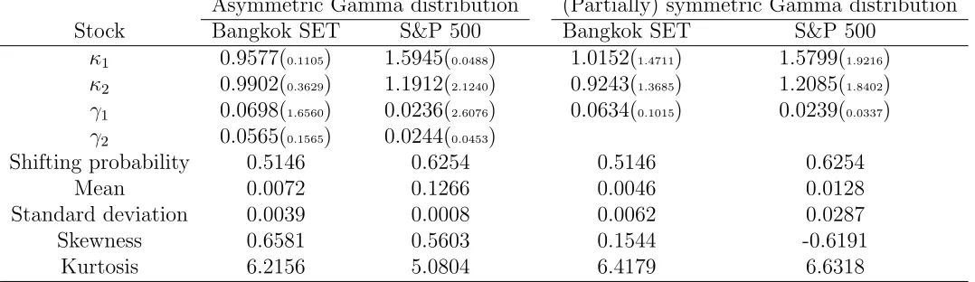
The ML estimates of the parameters of the return distributions for Bangkok SET and S&P 500 are reported in Table 4. The same phenomenon as shown in Table 3 can be noticed. That is, the mean and the standard deviation of S&P 500 are higher than those of Bangkok SET as shown in the second panel of Table 4. The skewness of S&P 500 is negative while it is positive for Bangkok SET. Moreover, the standard errors of the ML estimates in the (partially) symmetric case are in general smaller than those in the asymmetric case. This indicates that the asset returns are better modelled with a partially symmetric Gamma distribution. The type of symmetry can be further confirmed by the LR test as given in Table 5.
First, we choose a benchmark return (r) which must be less than the mean of the portfolio return (see Remark 2.1). Next, we estimate the optimal portfolios and the risk bounds that are the upper bounds of P{Rp,2(α)(ω) < r} for the models in Tables 1 and 2. Finally, we investigate the effect of the degree of absolute risk aversion, individual skewnesses and the nonlinear correlations on the optimal portfolio by examining the portfolio mean, the portfolio standard deviation, the portfolio skewness and the deviations function.
First, we shall assume that the asset returns are uncorrelated. The benchmark is set to -1%. Table 6indicates that for three modelsM1, M2, andM3, the proportion held in S&P 500 decreases as the degree of absolute risk aversion increases. Figure 5 shows that the growth rate (i.e., the deviations function) curve tends to shift upward as the degree of risk aversion increases. This implies that the risk bound decreases as an investor becomes more averse to the likelihood that the portfolio return underperforms a benchmark.
As shown in Table7, sinceM1 is the benchmark model, the pro of including the skewnesses is evident since the mean, the standard deviation, and the skewness of the optimal portfolio return in Model M2 are higher than those in Model M1. This is because the deviations function approximated with the third order Edgeworth expansion supports low standard deviation and positive portfolio skewness. However, in Model M3 where the exact mgf is used, the mean, the variance, and the skewness of the optimal portfolio return are less than those in Model M1. This is due to the presence of the high order moments which may dominate the low order moments, thus diminish the impact of the skewnesses. As a result, the high order moments decrease the mean, the variance, and the skewness of the optimal portfolio return whilst the individual skewnesses solely increase those of the optimal portfolio return. Hence, a rational investor prefers Model M2 to the other two models since this model gives a higher mean and a higher skewness at the cost of a slightly higher standard deviation.
Next, we assume that the asset returns are correlated. In this case, we need to make as-sumptions about the marginal return distributions and the portfolio return distribution. Suppose that the portfolio return distribution is an asymmetric Gamma distribution. The method proposed in Section 2.3 does not require us to estimate the measures of nonlinear correlation explicitly in order to estimate the optimal portfolio. Instead, the optimal port-folio is found by simultaneous maximization of the deviations function and the average log likelihood function.
than those inM1-M3 where asset returns are assumed to be uncorrelated. Thus, correlation apparently has a rather significant impact on optimal portfolio. By setting the benchmark return to -1% which is less than the sample mean of an asset return, we can observe that the optimal portfolio initially increases then decreases at the point where the degree of absolute risk aversion (θ∗) is 14.5 obtained by maximizing the deviations function w.r.t.
bothα and θ. As seen in Figures 6 and 7, the growth rate (the deviations function) curve for θ= 14.5 is on the top of the other curves. In another word, the optimal portfolio, that is a function of the degree of risk aversion, has smile shape. Furthermore, the risk bounds are much less than those inM1-M3. Thus, the modelsM4-M9 are much less risky than the models M1-M3. This is a benefit of asymmetric dependence in the portfolio analysis.
In addition, the effect of the nonlinear correlations on the optimal portfolio can be examined in Table7. In the asymmetric case,M4 is the benchmark model,M5, that is obtained by an application of the third order Edgeworth expansion of the exact mgf, yields a higher mean and a lower standard deviation at the cost of a lower skewness. Contrary to ModelsM1-M3, the presence of the second order nonlinear correlations as defined in Section 2.2 reduces the portfolio skewness whilst increasing the portfolio mean. In the symmetric case, M7 is the benchmark model, M8 yields a higher mean, lower variance, and a higher skewness. An interesting point to note is that the presence of the nonlinear correlations increases not only the portfolio skewness but also the portfolio mean. Since investors always prefer skewness, ModelM8 is obviously preferable to ModelM7. However, ModelM9, which uses the exact mgf, is the most favourable model since it gives a higher mean, a lower standard deviation, and a higher skewness. This is due to the fact that the high order correlations that combine with the second order nonlinear correlations support the deviations function to effectively generate a high mean, a low standard deviation, and a high skewness. Hence, the investment efficiency can be enhanced by incorporating high order correlations.
the optimal portfolio. First, we generate 2000 bivariate samples of two Gamma random variables with the true parameters as given in Table 4. Next, we use Model M6 or M9 to estimate an optimal portfolio by total maximization of the deviations function. The estimated optimal portfolio is then used to recover the linear correlation and nonlinear ones from each bivariate sample. Eventually, we have a sample of 2000 optimal portfolios together with recovered measures of correlation. As shown in Figure3, as the linear corre-lation increases, the proportion held in S&P 500 noticeably decreases. This is compatible with the results in Table 6 that when the asset returns are correlated, the proportion in-vested in S&P 500 decreases significantly. Now, we move on to examine Figure 4. When Model M6 is used, the nonlinear correlations (λ12) and (λ21), that are of different signs, have no effect on the optimal portfolio since they can be cancelled out, while the ones, that are of the same signs, have a rather strong effect as shown in Figure 5(a). However, when Model M9 is used, regardless of the signs, the nonlinear correlations always have a strong effect on the optimal portfolio as seen in Figure5(b). Thus, no effect of signs can be observed. This is due to the partial symmetry assumed for the portfolio return distribution. Hence, the sign effects of the nonlinear correlations are always stronger in the asymmetric case than in the partially symmetric case.
Therefore, the empirical results given in this section confirm our conjecture that asymmetric dependence between individual assets and asymmetry in the portfolio return are two typical types of asymmetry that have strong effects on optimal asset allocations. Moreover, we empirically show that highly efficient investment strategies can be devised by taking high order moments and high order correlations in to account. However, a general theory which can quantify the magnitude of effects is complicated to derive in our framework. This is an interesting topic for the future research.
4
CONCLUSION
maximizing the expected exponential utility function are satisfied. Then, we establish a theoreti-cal framework for finding optimal portfolios when there are many risky assets. However, because analysis of the effect of correlation on optimal portfolio is rather complicated for a large number of assets, we shall focus on the special case of two assets. An asymmetric Gamma distribution is used to capture two types of asymmetry; 1) asymmetry in the portfolio return distribution 2) asymmetric dependence (gauged by the second order measures of nonlinear correlation) between risky assets. Empirical evidences provided in Section 3 confirm that there is a strong effect of asymmetry and nonlinear correlations on optimal portfolio.
Appendix A. Proofs of results
The proof of Theorem 1 basically follows from the proof of Theorem 3.
Theorem 3. Let us define (n) IID random variables r˜i with the mgf mgf(θ), where i= 1, .., n.
The upper tail probability of rn= 1n"ni=1˜ri is given by (A.36) or (A.37). That is,
P{rn> r}%
1 √
2πnθ(r)σ(r)exp{−nΛ(r)}, (A.36)
where σ2(r) = 1
θ!
(r) )
= Λ”1(r) *
, Λ(r) = supθ>0
-θr−logE[exp{θr˜1}] .
, andθ(r) = arg supθ>0
-θr−
logE[exp{θr˜1}] .
.
P{rn > r}= exp{−nθ(r)}exp -1
2nσ
4(r)θ2(r).#1
−mgf'√nσ2(r)θ(r)(&'1 +op(1) (
. (A.37)
Proof. See Zhulenev (1997).
Remark 4.1. Let θ+ = sup{θ ∈ (0,∞) : mgf(θ) < ∞} and r+ = limθ−→θ
+{ mgf!(θ)
mgf(θ)}. Since Λ!
(r) =θ(r)+θ!
(r)-r−mgf !
(θ(r)) mgf(θ(r))
.
. Ifr =E[˜r1] thenθ(E[˜r1]) = 0sincelog '
mgf(θ)(is a strictly convex function (i.e., Λ(r) is a strictly concave function.) Therefore, for anyr ∈(E[˜r1], r+), the maximal value of Λ(r) is attained at a unique point θ(r), where the tangent line to mgf(θ(r))is parallel with the line rθ. Moreover, the function θ(r) increases ∀ r ∈(E[˜r1], r+). Further results can found in Zhulenev (1997).
Proof of Theorem 1. Now, we give a proof for the upper tail. The proof of the large deviations
result for the lower tail is quite similar. The portfolio return is given by
R(α) p,n(ω) =
n 2
i=1
αi˜ri, (A.38)
An application of Cramer’s transformation yields
P{R(α)
p,n(ω)> r}=mgf '
θ(r)( H
∞
r
exp{−θ(r)u}P{R(α,r)
p,n (ω)∈du}, (A.39)
whereR(α,r)
p,n (ω) is a weighted sum as (A.38) with the mean (r) and the variance (σ2(r)). mgf(θ) is the mgf of R(α)
p,n(ω) and θ(r) = argsupθ>0 #
θr−logmgf(θ)&. [Note that since mgf
!
(θ)
mgf(θ)|θ=0 =µ, thus if r=µthen θ(r) = 0.] Hence, we have
P{R(α)
p,n(ω)> r} = mgf '
θ(r)( H
∞
0
exp{−θ(r)(u+r)}P{R(α,r)
p,n (ω)∈r+du} = mgf'θ(r)(exp{−rθ(r)}
H ∞
0
exp{−θ(r)u}P# R
(α,r)
p,n (ω)−r 1"n
i=1α2iσ(r)
∈ 1"ndu i=1α2iσ(r)
&
= exp-−'θ(r)r−logmgf(θ(r))(. H ∞
0
exp#−θ(r) I J J K2n
i=1
α2 iu
&
P# R
(α,r)
p,n (ω)−r 1"n
i=1α2iσ(r)
∈du&.
Applying the integral separation formula forF(r)(u) =P# R(
α,r) p,n (ω)−r √ n
i=1α2iσ(r)
≤u&, we have
P{R(α)
p,n(ω)> r}=θ(r)σ(r) I J J K n 2 i=1 α2 i exp #
−)θ(r)r−logmgf'θ(r)(*&
H ∞
0
exp#θ(r)σ(r) I J J K2n
i=1
α2 iu
&'
F(r)(u)−F(r)(0)(du. (A.40)
Moreover, an Edgeworth expansion of dF(r)(u) yields
dF(r)(u) = P# R
(α,r)
p,n (ω)−r 1"n
i=1α2iσ(r) =u&
= φ(u)− E $
R(α,r)
p,n (ω)−r%3 '
E[R(α,r)
p,n (ω)−r]2( 3 2
φ!!!(u) + remainder,
the approximation of dF(r)(u) in to (A.40), we have
P{R(α)
p,n(ω)> r} = β(r) exp #
−)θ(r)r−logmgf'θ(r)(*&# H
∞
0
exp{β(r)u}'Φ(u)−Φ(0)(du
− E[R (α,r)
p,n (ω)−r]3 '
E[R(α,r)
p,n (ω)−r]2( 3 2
H ∞
0
exp{β(r)u}'Φ(3)(u)−Φ(3)(0)(du&+ remainder,
whereΦ(u) is the lower tail of the standard normal distribution,Φ(3)(u) is the lower tail ofφ!!!
(u), and β(r) =θ(r)σ(r)1"ni=1α2
i.
In view of
H ∞
0
exp{θu}exp-− u 2
2 .
du=√2πexp-θ 2
2 .'
1−Φ(θ)(,
we can easily derive H ∞
0
exp{β(r)u}'Φ(u)−Φ(0)(du = 1
β(r) )
exp-β 2(r)
2 .'
1−Φ(β(r))(*,
H ∞
0
exp{β(r)u}'Φ(3)(u)−Φ(3)(0)(du = exp-β 2(r)
2 .)
1−Φ'β(r)(*'β2(r) + 2(
+ √1 2π
)
β(r) + 1
β(r) *
.
Hence, we obtain
P{R(α)
p,n(ω)> r} = β(r) exp{−Λ(r)}
#exp{β2(r) 2 }
$
1−Φ'β(r)(%
β(r) − E[R
(α,r)
p,n (ω)−r]3 [E[R(α,r)
p,n (ω)−r]2] 3 2 +
exp-β 2(r)
2 .$
1−Φ(β(r))%$β2(r) + 2%
+ √1 2π
)
β(r) + 1
β(r) *,
+ remainder&, (A.41)
where Λ(r) =θ(r)r−logmgf(θ(r)).
Since ("ni=1α2i)32 ≥ "n
i=1α3i then "n
i=1α3i approaches to zero faster than ( "n
i=1α2i) 3
2 as (n) is sufficiently large. Furthermore, since all the central moments of ˜r1 are finite, it follows that
E[R(α,r) p,n (ω)−r]3 [E[R(α,r)
p,n (ω)−r]2] 3
(A.41) is negligible. Therefore, (A.41) can be written as
P{R(α)
p,n(ω)≥r}≈exp{−Λ(r)}exp
-β2(r) 2
.$
1−Φ'β(r)(%+o(1).
Furthermore, by the approximation
1−Φ'β(r)( = exp{−
β2(r) 2 } 1
2πβ(r) ,
we obtain the main result of Theorem 1. Finally, in order to show that σ2(r)2 = 1
Λ”(r) we make use of the following identity:
Λ!
(r) =θ(r),
mgf!(θ) mgf(θ) 4 4 4
θ=θ(r) =r. (A.42)
Take the first derivative of (A.42) w.r.t. (r), we have $
mgf”'θ(r)(mgf'θ(r)(−'mgf!'
θ(r)((2%θ!(r)
mgf2'θ(r)( = 1
⇔
mgf”(θ)mgf(θ)−'mgf!(θ)(2
mgf2(θ)
4 4 4
θ=θ(r) = 1
θ!
(r).
Since log'mgf(θ)(444
θ=θ(r) =r=E[˜r1], we obtain σ
2(r) = log”'mgf(θ)(44 4
θ=θ(r) = 1
θ!
(r) )
= 1
Λ!!
(r) *
.
Proof of Theorem 2. Given the probability space 'Ω,{Fn}∞
n=1 (
that generates the portfolio returnR(α)
p,n(ω), where (ω) is used to emphasize thatR( α)
p,n(ω) is a random variable, (n) is used to stress thatR(α)
p,n(ω) depends on (n), and (α) is used to denote thatR(
α)
• UPPER BOUND: Since
{ω ∈Ω: R(α)
p,n(ω)≥r}≡
-ω∈Ω: exp{nθR(α)
p,n(ω)}≥exp{nθr} .
∀ θ >0,
then an application of the Tchebyshev inequality yields
P{R(α)
p,n(ω)> r} ≤ P
-exp{nθR(α)
p,n(ω)}>exp{nθr} .
≤ exp{−nθr}E$exp{nθR(α) p,n(ω)}
%
.
Hence, we have
lim sup n−→∞
1
nsupα∈S
logP{R(α)
p,n(ω)> r}≤− lim sup n−→∞
1
nαinf∈S )
nθˆr−logE[exp{nθˆR(α) p,n(ω)}]
*
,
where S is a compact set of feasible investment and ˆθ is in the neighbourhood of
θ∗ = lim n−→∞
1
n αinf∈S sup
θ∈(0,∞) )
nθr−logE[exp{nθR(α) p,n(ω)}]
*
.
• LOWER BOUND:This part uses the Randon-Nykodym theorem and the Borell-Catelli
lemma.
First, let us define another probability measure Q on the probability space (Ω,{Fn}∞n=1) such that
dQ dP
4 4 4
Fn def
= exp#nθˆR( ˆα)
p,n(ω)−logE[exp{nθˆR( ˆ α) p,n(ω)}]
&
,
where
ˆ
α(ˆθ, n) = arginf
α∈S )
nθˆr−logE[exp{nθˆR(α) p,n(ω)}]
*
.
Next, since {ω ∈ Ω : R( ˆα)
p,n(ω) > r −-} ⊇ {ω ∈ Ω : r−- < R( ˆ α)