Enhanced imaging of metallic knee prostheses by using a representative phantom

(1)

1

ENHANCED IMAGING OF METALLIC KNEE

PROSTHESES BY USING A REPRESENTATIVE

PHANTOM

R.P.A. Boekestijn, R.J. van Dijk, T.M.N. van Helden, R. Hoogland

Multidisciplinary Assignment

Bachelor Technical Medicine

June 2016

Technical supervisor:

J.K. van Zandwijk, MSc

Medical supervisor:

Dr. R. Huis in’t Veld

Process supervisor:

(2)

(3)

3

Preface

The writing of this study has been performed in order to get our Bachelor's degree of Technical Medicine. It gives us the opportunity to implement our knowledge gained during our bachelor program. We would like to thank our supervisors who were always willing to help when we needed some assistance. We expanded our knowledge during this research both in personal development and regarding research skills and had fun while doing so. Enjoy reading our paper!

We want to thank the following persons for guidance during the multi disciplinarily assignment: J.K. van Zandwijk, MSc (Technical Supervisor)

(4)

(5)

5

Abstract

Objective: Investigate how a representative phantom can contribute to enhanced imaging of a Total Knee Arthroplasty (TKA) prosthesis in low-field MRI.

Method: Ingredients of the phantom are gelatine (gelling agent), Dotarem® (T1 modifier), agarose (T2 modifier) and demineralised water. The T1 and T2 relaxation times of tissue mimicking samples are measured using a spin echo sequence in a 0.25 Tesla low field MRI. Artefacts sizes in the MR images of the phantom materials with prosthesis are measured and compared with the artefact sizes in the MR images of a human knee with prosthesis.

Results: Relaxation times of the samples ranged from 210 to 480 for T1. It was not possible to calculate T2 values in the samples. The artefact sizes differ from artefacts in a real knee with prosthesis. Relaxation times of the human knee ranged between 160 and 470 for T1 and between 25 and 127 for T2.

The phantom is not representative for a human knee, the images do not match. Comparison between phantom with prosthesis and knee with prosthesis show conflicting results. Especially the FSE X-MAR scan of the phantom shows more artefacts than the standard FSE scan.

Conclusion: It was not possible to create a representative phantom. It is seen that Dotarem® and agarose change T1 relaxation times. The metal artefacts do not show consistent results. For further research a more realistic phantom is needed to get comparable distortion in surrounding tissues. A representative phantom with complex structures should determine in what way metal artefacts can be reduced, to better image TKA problems.

(6)

(7)

7

List of abbreviations

Abbreviation Definition

CT: Computed tomography

FOV: Field-of-view

FSE: Fast spin echo

MOLLI: Modified look-locker inversion recovery

MRI: Magnetic resonance imaging

OCON: Orthopedisch Centrum Oost Nederland

PD: Proton Density

PJI: Prosthetic Joint Infection

RF: Radio Frequent

ROI: Region of Interest

SE: Spin Echo

SNR: Signal to noise ratio

TE: Echo time

TKA: Total Knee Arthroplasty

(10)

(11)

11

Introduction

Osteoarthritis is a disease that affects the cartilage in the joints. When this cartilage breaks down, it leads to pain and stiffness. In 2011, 227.000 men and 367.000 women are diagnosed with knee osteoarthritis in the Netherlands. [1] In 2014 24.057 of these patients in the Netherlands were treated with a total knee arthroplasty (TKA). [2] A TKA prosthesis consists of three parts: a tibial plateau, a femoral part and a sliding layer between these two. When the backside of the patella is worn, a fourth part is added at the backside of the patella. [3]

Once applied into the body, a TKA prosthesis last for 15 to 20 years, depending on usage. In some cases, however, the prosthesis has to be revised sooner because it wears faster than expected or it detaches from surrounding structures.[4] In 2014 2.541 revisions took place in the Netherlands. [2]

The most common indicators for a revision surgery are instability of the TKA prosthesis, stiffness after a TKA surgery, aseptic loosening and peri-prosthetic joint infection (PJI). [5] In order to visualize these complications plain films, nuclear scanning, Computed Tomography (CT) or Magnetic Resonance Imaging (MRI) can be used. [6] As this study focusses on MRI, the other techniques will not be further elaborated. However, MRI has its shortcomings. A limitation of MRI is that the presence of metallic objects lowers the imaging capabilities of MRI. [7,8] As the TKA prosthesis is ferromagnetic, it will disturb the magnetic field of the MRI (B0). [9] The size of the artefact increases with the field strength of the MRI, thus the prosthesis

is possibly better imaged with low-field MRI. [10]

Research should determine how low-field MRI can be used to image patients with a TKA prosthesis. In order to do this as efficiently and effectively as possible, such research often uses phantoms. In order to make a good, accurate comparison with human tissue, researchers need a phantom that is close to a natural knee in low-field MRI. The requirements of a useful phantom are: [11,12]

1. Available 2. Inexpensive 3. Easy to handle

4. Easy to edit in different shapes 5. Durable

6. Harmless

7. Similar in relaxation times to bone marrow, fat or muscle

(12)

12 This research uses Gadolinium (in Dotarem®) and agarose as T1 and T2 modifiers to vary the phantom's relaxation times. Paramagnetic Gadolinium ions lower the T1 relaxation time. The benefit of Gadolinium over copper is that Gadolinium is not influenced by temperature or magnetic field strength. [12,15] Agarose lowers the T2 relaxation time. It is beneficial for its dissolving qualities. Whereas other potential fabrics like graphite and aluminium powder precipitate, agarose homogeneously dissolves into the phantom. Another benefit of agarose is that it adds some strength to the phantom, because of its gel-like characteristics. [13,16] Gelatine is used, as it was directly available.

(13)

13

Objective

This research is part of a larger overall research of enhanced imaging of patients with metallic knee prostheses. This research has two primary goals:

1. Finding materials that are representative for human tissue in low-field MRI

2. Figuring out the effect of prosthetic material on the representative materials in low-field MRI. The main question that will be answered is:

How can a representative phantom for patients with metallic knee prostheses contribute to enhanced imaging of these patients with low-field MRI?

This question will be answered using the following sub questions:

 Which concentrations of the phantom materials represent bone, muscle and fat tissue in the human knee according to literature?

 How to calculate T1 and T2 relaxation times?

 Which concentrations of the phantom materials represent bone, muscle and fat tissue in the human knee during a low-field MRI scan?

 How to quantify the size and distortion of metal artefacts in low-field MRI?

 What is the difference in size and distortion of the metal artefacts in low-field MRI between the phantom (with prosthesis) and a human knee (with prosthesis)?

Hypothesis

(14)

(15)

15

Background information

Anatomy

The human knee consists of three bones: the femur (thigh bone), tibia (shin bone) and the patella (kneecap). Although the fibula (calf bone) is located close to the knee joint, it is not actually part of the joint. All places of contact within the knee joint are covered with cartilage. Between the femur and the tibia are two menisci (lateral and medial meniscus) that reduce friction and absorb some of the shocks the joint may encounter. The bones are encapsulated by the fibrous and synovial membrane. Inside this membrane synovial fluid makes sure that the joint keeps lubricated.

A series of ligaments and tendons stabilize the joint and hold all the separate parts together. The extracapsular ligaments are located on the outside of the joint. The patellar ligament is located on the anterior side of the knee. Laterally and medially to the knee joint are the collateral ligaments (fibular collateral ligament and tibial collateral ligament). The oblique popliteal ligament and arcuate popliteal ligament are the two ligaments strengthening the posterior side of the knee. [17]

The two ligaments inside the knee joint are called cruciate ligaments. They are located in the middle of the joint and cross each other forming the letter 'X'. They prevent cruciate ligaments are the two ligaments inside the knee joint. They lay in the middle of the joint and cross each other forming the letter X. They prevent anterior and posterior movement of the femur and tibia. Some of the muscles surrounding the knee also play a role in stabilizing the knee-joint (Figure 1). [17]

FIGURE 1:ANATOMY OF THE KNEE, FRONTAL VIEW [18]

Pathology

(16)

16 In most of the cases, arthritis is age-related. Other causes of the disease are bone damages, previous knee surgeries, inflammations and infections. Risk factors for the development of arthritis are obesity, performing a heavy job, the position of the legs and heredity. [19]

Total Knee Arthroplasty

A TKA surgery in which an arthritic knee is replaced by a prosthesis follows an eight-step procedure (Figure 2). After opening the knee and setting the joint, pieces of the femur and tibia are removed using a template. Hereby, the anterior cruciate ligament and lateral cruciate ligament are removed as well. After the bone has been prepared, the metal implants are secured into the bone using cement or pressure. After that, plastic is placed between the metal parts, in order to create a gliding surface. [3,20]

FIGURE 2:STEP-BY-STEP OVERVIEW OF THE PROCEDURE OF A TKA SURGERY [3]

TKA failures

After surgery different failures of TKA prosthesis can cause patient's discomfort. A revision of the TKA is often necessary to help a patient. The most common failures are:

 Instability of the TKA prosthesis. Most of the time, patients do not feel the instability. They only feel pain and sometimes functional impairment due to the instability. Risk factors for getting an instable knee prosthesis are: obesity, muscular pathologies, hip or foot deformities and neurologic pathologies.

 Stiffness after a TKA surgery. The flexion and extension of the knee are substandard, what causes pain. Risk factors for this problem are a limited range of motion before surgery, a poor recovery after surgery, biological predisposition, intraoperative complications and psychological problems of a patient.

 Aseptic loosening. Most of the time, this is implant-related. A big risk factor for this problem is obesity. Other risk factors are material debris in the knee and a malalignment of the leg. Patients feel pain during walking and weight-bearing.

(17)

17

Basic principles of MRI

In theory many of the chemical elements that make up our bodies can be used for MRI scans. However, MRI technology uses hydrogen atoms as they are abundant and have a large gyromagnetic ratio. Large parts of bodies consist of water. The chemical consistency of water (H2O) has two hydrogen atoms and one oxygen atom, so there are a lot of hydrogen atoms in our body that an MRI scanner can use. The gyromagnetic ratio of hydrogen is 42.57 MHz/T, which is ideal for imaging.

Hydrogen atoms contain a single positively charged proton and a single negatively charged electron. The proton is like a little magnet with a north and a south pole. As the proton is charged, turns around its axis. MRI technology uses the magnetic properties of the protons in hydrogen atoms to create a signal. A MRI scanner applies a strong magnetic field (B0) to the patient, at which the hydrogen protons align, either parallel or anti-parallel, with magnetic field B0 of the MRI. This affects the protons in two ways: their axes

turn and point along the field direction and they precess around B0 with the Larmor frequency. The

magnetic fields of all protons added together referred to as net-magnetisation.

The signal of the MRI is measured by induction. The signal is detected by a receiving coil. When no scanning is taking place, the net-magnetisation is aligned with the main magnetic field B or the Z-axis. The MRI coils then do not measure anything. A signal can only be measured when the magnetisation is turning through the coil. When a radio frequent pulse (RF) is applied, the net-magnetisation is tipped out of alignment into the xy-plane. When protons are excited by the RF frequency, they are in a high-energy state. They want to return to their natural low-energy state, so when the RF frequency is removed, they return to the direction of B0. The process is called relaxation. T1 relaxation describes what happens along the z-axis (Figure 3). [21]

FIGURE 3:T1 RELAXATION, AFTER THE RF EXCITATION PULSE THE NET MAGNETISATION RAISES ALONG THE Z-AXIS [22]

(18)

18

FIGURE 4:T2 RELAXATION, THE NET MAGNETIZATION VECTOR TURNS IN THE XY-PLANE AND TURN OUT PHASE [22]

Every tissue has its own values for T1 and T2, because protons are bounded differently in every molecule. [21]

During the relaxation process the spinning protons exude their excess energy in the form of radio frequent-waves. These waves can be measured when they are perpendicular to the main electric field and can only be measured over a short period of time. [21]

In order to localise these signals three additional magnetic gradients are applied. These gradients are generated by three coils in the directions z, x and y. [21]

 The z-gradient defines the difference along the main magnetic field. The magnetic field is higher at the top and lower at the bottom. A higher magnetic field B0 means a higher Larmor frequency. The protons will spin with a different frequency. By using a RF pulse with a higher frequency the protons in the top of the body will react because they are the only ones that are spinning at that frequency. In this way, a body slice is selected.

 The y-gradient defines the phase (point on the circle of a waveform). The protons in the anterior part of the slice will turn faster than the protons in the posterior part of the slice. The moment the gradient is switched off, the protons will spin with the same velocity, but at a different phase.

 The x-gradient defines the frequency. The protons on the left will turn with a different frequency than on the right. This frequency difference will result in a phase difference that can later be used for localisation. The lower frequency protons will get an extra phase difference on top of the phase difference created by the y-gradient.

Combined the three gradients form unique combination of frequency and phase, localising the signal to a specific voxel (point in space).

(19)

k-19 space is almost symmetric from top to bottom. That means that if a little more than 50 percent of the data is known, the rest of the k-space can be filled in based on the symmetry. The K-space is not perfect symmetric, filling the k-space based on symmetry is only used by fast scanning. [22]

In order to improve the signal of an MRI scan, the Spin Echo sequence (SE) can be used (Figure 5). With a 90 degrees’ excitation pulse the net magnetisation is flipped towards the xy-plane. After that, the signal dephases as a result of T2 relaxation. SE sends an additional RF pulse, this time a RF pulse of 180 degrees. As a result, the spins rephase and produce a higher signal. This signal is an echo, because it is reconstructed out of the original signal (Figure 6). [21]

FIGURE 5:SPIN ECHO SEQUENCE [22]

FIGURE 6:REPHASING OF THE SIGNAL, SPIN SYSTEM FLIPPED OVER THE Y-PLANE [22]

In order to fill the k-space this process is repeated until the matrix is filled. The repetition time (TR) is the time between two 90 degrees excitation pulses. The echo time (TE) is the time between the 90 degrees excitation pulse and the echo. [21]

In addition to high-field MRI there is low-field MRI. The difference between the two is that low-field MRI uses a lower magnetic field B0. High-field MRI units provide better spatial and contrast resolutions [23].

The use of low-field MRI however has several advantages over high field MRI: [24]

 The open design of low-field MRI maximizes patient comfort and minimizes claustrophobia.

 Some systems are able to turn to a 90 degrees angle, which allows the user to take gravity into account.

 The low-field MRI may cost only half that of a high-field MRI because purchase price increases with field strength

(20)

20

 Low-field MRI has a lower fringe field, which means it is easier to site and shield the magnet within a hospital or imaging centre.

 Low-field MRI is less susceptible to metal artefacts because the difference in signal strength is highlighted to a smaller degree than it is in high-field MRI. The artefact size is proportional to the field strength. This means that MRIs with lower field strength have smaller artefacts than high-field MRIs.

 Lower energy deposition in tissues. Energy deposition causes tissue heating, which is dangerous. The amount of energy deposition in tissue by radio frequent pulses is proportional to the square of the magnetic field strength. [25,26]

MRI artefacts

When imaging with MRI, artefacts are always present. Artefacts are misrepresentations of the object or distortions in the image and can make it difficult to differentiate structures. In order to interpret the images accurately, it is necessary to understand what kind of artefacts can occur with MR imaging. Artefacts are divided in three main groups: tissue-, motion- or technique-related artefacts. In this research the focus will be on the tissue-related artefacts, specifically the metal artefacts. Those artefacts are the most important since they distort the image the most. Tissue artefacts are: chemical shift, chemical shift 2nd kind (India ink), magic angle, dielectric and the magnetic susceptibility artefact. The following technique related artefacts are discussed: aliasing, truncation and RF overflow artefacts. [27]

Small local differences in magnetic shielding of electron clouds are present between water and fat molecules. This results in a small frequency shift, which makes the spatial position shift and will show the fat or water protons mismapped on the MR image in the frequency-encode direction. This occurs because the MRI scanner perceives the fat samples as if they are water molecules from a different voxel and is called a chemical shift artefact. Chemical shift of the 2nd kind will not occur with spin echo sequences, but only occur with gradient echoes, which will not be used in this research. [28,29]

Magnetic susceptibility artefacts occur when the main magnetic field is disturbed by a magnetized material. This disturbance causes distortions in both the frequency and phase encoding direction. Materials that can disperse the magnetic field are called diamagnetic. While materials that can concentrate the magnetic field are called (super)paramagnetic or ferromagnetic depending on the size of the caused effect. Ferromagnetic materials cause the largest artefacts and are thus the biggest problem. The artefact size is proportional to the field strength as well, therefore low-field MRI should improve imaging in patients with metal implants over high-field MRI. [30]

The magical angle artefact occurs when highly-structured molecules, like collagen, are imaged under a 54,7 degree angle. This increases the intensities of the processed MRI signal at places where it should not and makes certain structures look pathologic when they are not. Since such information will not be processed in this research, it should only be taken into account when collecting the healthy values.

(21)

21 The technique related artefacts can mostly be prevented by calibrating the MRI scanner and following the right scan protocols. The herringbone or shading artefact should be taken into account which can be caused by power spikes and the patient touching the RF coils. [31]

A common software artefact is aliasing (or wrap-around artefact). This occurs when the field of view (FOV) is smaller than the body part being imaged. The FOV is assigned with 360 degrees of phase cycles. When an object falls outside this FOV it will be assigned a degree above or below 360 degrees. Since the phase-encoding step defines all spatial positions in the 0 to 360 degree range, this means that an object with 361 degrees is perceived as 1 degree and will be mismapped on the other side of the image. [29]

Another software artefact is the truncation artefact. This artefact is characterised by lines running parallel to an object with sharp high-contrast boundaries. It originates in the conversion between scanning and reconstruction because the software is not able to reconstruct this sharp contrast. [31]

(22)

(23)

23

Method

Phase I material concentration research

I.A Preparation of material samples

This research uses a phantom composed of gelatine (Dr. Oetker), agarose (Invitrogen, UltraPure), Dotarem® (Guerbet) and demineralised water.

For the study 27 samples are produced where each sample consists of 10 gram gelatine, a concentration of agarose between 1.0-3.5 mg, a concentration of Dotarem® between 0-4.5 µL and 90 gram distilled water.

Table 4 (Appendix A) indicates the exact concentrations for each sample. In order to measure the quantities of all substances a scale with an accuracy of 0.001 gram is used. A pipette of 2-20 µL is used for the measurements of Dotarem®.

The selected concentrations of agarose and Dotarem® are based on a previous study by Yoshimura et al.. [12] Yoshimura et al. used GdCl3 as T1 modifier instead of Dotarem®. We converted the concentrations of GdCl3 to concentrations of Dotarem® by using the molecular weight of the elements. The used converting formula is shown in equation 1. [12]

𝐷 =[𝐺𝑑] ∗ (𝑆𝑊) ∗ 𝑀 ∗ 10

−7

𝐶 ∗ 10−3 (𝑒𝑞𝑢𝑎𝑡𝑖𝑜𝑛 1)

The formula uses the following variables as input variables:

 D = the amount of Dotarem® in mL

 [Gd] = the amount of GdCl3 in µmol/kg, used in previous study

 SW = Sample weight (100 gram)

 M = molecular weight of Dotarem® (558.64 g/mol)

 C = concentration of Gd in Dotarem® (279.32 mg/mL)

All substances are mixed together in a beaker. The mixture is heated until 90-100 °C while being stirred in order to dissolve the gelatine and agarose. Gelatine dissolves at +- 40 °C and agarose at 90-100 °C. [33] After heating, the mixture is placed in a test tube and sealed with a stop. As a last step, the mixture is placed in a fridge of +-5 degrees for at least two hours.

I.B MRI measurements

The MRI measurements are made with a 0.25T low-field MRI scanner of Esaote, model G-scan Brio. For all measurements the DPA knee coil (elliptical 143x160x183 mm) is used.

(24)

24 The DPA knee coil is open, that is to say it has two open ends. After some tests the signal to noise ratio (SNR) at the open ends of the coil turned out to be lower than the SNR in the centre of the coil. In order to make sure that every sample is scanned with the same SNR, all samples were placed in a circle-formation in the centre of the coil. We used a transverse scanning plane to scan our samples. We placed markers to locate the samples.

The samples are scanned with the lowest possible slice thicknesses (2 mm and 3 mm) in order to get an accurate image. A large thickness has a negative effect on the detail of the MR image, because the average of a larger tissue portion is taken. In order to be able to make a reliable comparison, all other settings were kept the same, such as matrix (256x61), field of view (FOV)(250x120), band width and number of acquisitions (1), fixed at each scan.

For T1 calculation a 0° spin echo sequence is used. The TE is fixed at 18 ms and the TR values varied with: 50, 120, 190, 260, 330, 400, 470, 540, 610, 680, 750, 890, 1030, 1170, 1300 and 1500 ms. The shortest TE of the system is chosen in order to make T2 influence minimal. TR times are chosen in steps between 50 and 1500 in order to make an accurate estimation of the T1 relaxation curve. [12,13]

For T2 calculation a 0° spin echo sequence is used. The TR is fixed at 2500 ms and TE varied with: 18, 24, 30, 34, 50, 80, 90, 100, 110 and 120 ms. In order to eliminate most of the T1 influence, almost all longitudinal magnetization should be recovered. About 3-5 times of the T1 time are needed for such recovery (T1 interval times). Table 1 shows that increasing the number of T1 intervals above 4.0 makes the regrowth of the net magnetisation is neglectable. However, when a very high TR is chosen, the scan time increases significantly. TE times are chosen in steps between 18 and 120 in order to make an accurate estimation of the T2 relaxation curve. [34]

TABLE 1:PERCENTAGE OF NET MAGNETISATION (MZ) NEXT TO AMOUNT OF T1 INTERVAL TIMES REQUIRED TO GET THAT PERCENTAGE OF MZ REGROWTH [21,35]

Amount T1 times

Regrowth of longitudinal magnetization

0.5 39%

1.0 63%

1.5 78%

2.0 86%

3.0 95%

4.0 98%

5.0 99%

In order to validate the T1 and T2 values a healthy knee is scanned with the same settings as the samples. Homogeneity test

(25)

25

FIGURE 7:GELATINE SAMPLE WITH POSITIONS OF ROIS MEASURED FOR THE HOMOGENEITY TEST

I.C Examination of relaxation times

The MRI measurements were analysed using MATLAB R2016a software. In order to determine the sample intensities, a ROI was taken from each sample and the mean calculated with MATLAB R2016a. We made a correction for the background intensity of the MR images, as the intensities differed across the image we generated. We used the following formula to calculate the intensity:

𝐼𝑛𝑡𝑒𝑛𝑠𝑖𝑡𝑦 = 𝑚𝑒𝑎𝑛 (𝑅𝑂𝐼 𝑠𝑎𝑚𝑝𝑙𝑒) − 𝑚𝑒𝑎𝑛 (𝑅𝑂𝐼 𝑏𝑎𝑐𝑘𝑔𝑟𝑜𝑢𝑛𝑑) (𝑒𝑞𝑢𝑎𝑡𝑖𝑜𝑛 2)

The T1 relaxation time is calculated by plotting the reduced intensities against the TR. For the T2 relaxation time the reduced intensities are plotted against TE. The fit function in MATLAB R2016a plotted a predicted exponential curve through the intensities. The T1 value is the value at 63.2% at the intensity/TR curve and the T2 the 36.8% value at the intensity/TE curve. (Figure 8) [36–38]

FIGURE 8: A (LEFT): AN INTENSITY CURVE FOR CALCULATION OF T1 RELAXATION TIMES.B(RIGHT): AN INTENSITY CURVE FOR CALCULATION OF T2 RELAXATION TIMES

Statistics

(26)

26

𝜎 = √( 1

𝑁 − 1) ∑|𝐴𝑖− 𝑥̅|

2 𝑁

𝑖=1

(𝑒𝑞𝑢𝑎𝑡𝑖𝑜𝑛 3)

𝑥̅ − 𝑧 ∗ 𝜎

√𝑁≤ 𝑥̅ ≤ 𝑥̅ + 𝑧 ∗

𝜎

√𝑁 (𝑒𝑞𝑢𝑎𝑡𝑖𝑜𝑛 4)

Phase II Metal artefact research

II.A Preparation of phantom with prosthesis

In order to explore the influence of agarose and Dotarem® on the size of metal artefacts, we created a phantom with two stacked layers. The first layer consisted of 10 % gelatine and the second layer consisted of 10 % gelatine, 2 gram agarose and 3 µL Dotarem®. In the centre of the phantom a femoral Co-Cr part of a prosthesis is placed. The sizes of the femoral part are measured with a calliper. Figure 9 shows the measured parts.

FIGURE 9:SIZE MEASUREMENTS OF PROSTHESIS

II.B MRI measurements

The phantom is scanned with the MRI settings listed in Table 2. [39] In order to validate the artefact size of the phantom, a participant with a prosthesis is scanned with the same settings. The TKA of the participant consists of a titanium (Ti-6AL-4V) tibial plateau, a femoral part made of Co-Cr and two sliding layers of polyethylene. [40]

TABLE 2:SETTINGS OF THE MRI SCANNER FOR EACH SEQUENCE

Sequence FSE PD X-MAR FSE PD Fast STIR X-MAR FAST STIR XBONE T2

Orientation sagittal sagittal coronal coronal coronal

Thickness 4 4 4 4 4

Bandwidth 10.3010 10.3010 10.3011 10.3011 10.3010

FA 90 90 90 90 45

Matrix size 288x240 224x224 224x218 240x228 288x224

Number of acquisitions

2 1 2 1 1

TR 2860 2560 2740 2580 900

TE 12 25 12 25 14

TI - - 75 70 -

(27)

27

II.C Examination of metal artefacts

RadiAnt DICOM viewer 3.0.2. is used for the measurement of the artefact sizes. We made the assumption that the artefact follows the contour of the prosthesis. The contours are determined by human sight and then measured with the measuring tool in RadiAnt. The distances between the femoral condyles

(28)

(29)

29

Results

Phase I material concentration research

I.B MRI measurements

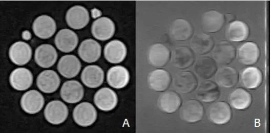
Figure 10 displays the MR images used for the calculation of the T1 and T2 relaxation times of the scanned samples. In both images some inhomogeneity of the samples is shown by darker and lighter spots. The MR images of the T2 sequences with TE times above 80 ms differ from all the other T2 images. The intensity of the background of the images with TE times above 80 ms is high, which resulted in a grey background. Besides the intensities of the samples are not in line with the other measured sample intensities for the T2 relaxation time. This looks like an RF overflow artefact. [41]

The MR images used for the calculation of the T1 relaxation times of the scanned samples (Figure 10)Figure 1 show the same inhomogeneity. In most of the samples an artefact can be seen. Samples show oval lines disturbing the homogeneity in each sample. The high intensities shown in Figure 10B are not found in the MR images for the calculation of the T1 relaxation times.

In Figure 11 a scan of the healthy knee used for the validation of the T1 relaxation time and T2 relaxation time calculations is shown. The bone, muscle and fat structures of the knee are possible to distinguish, which is desirable for further analysis. Parts of the knee closer to the open ends of the coil show a lower intensity, which can be seen in the darker image. In the MR images used for calculating the T2 relaxation time of the knee tissues, an aliasing artefact is shown. [29]

FIGURE 10A.AN MR IMAGE USED TO CALCULATE T1 TIMES,THICKNESS 3 MM,TR1500 MS;B.AN MR IMAGE USED TO CALCULATE T2 TIMES, THICKNESS 3 MM,TR2500 MS,TE90 MS

[image:29.595.74.340.307.438.2]

(30)

[image:30.595.74.414.167.375.2]

30 Homogeneity test

Figure 12 shows the intensity for each ROI in the gelatine sample (Figure 7). A variation in intensities is seen, by comparing the intensities at each location. From the top to the bottom of the gelatine sample. (ROI: 1-7) the values seem more or less the same, with a 95% confidence interval of (1065.26-1113.92). From the left of the gelatine sample to the right of the sample (ROI: 8-10, 4, 11-13) inhomogeneity is seen, with a 95% confidence interval of (1091.15-1266.16).

FIGURE 12RESULTS OF THE HOMOGENEITY TEST OF GELATINE SAMPLES.INTENSITIES OF ROIS

I.C Examination of relaxation times

The calculated T1 and T2 values of bone, muscle and fat knee tissues of the healthy knee, used for the validation of the T1 and T2 relaxation time of the samples, are displayed in Figure 13Figure 13. Remarkable is the difference between the relaxation times of femur and tibia bone tissue, which is 54 ms. The values found in the literature are slightly different than the measured values. [22] Despite the difference we used the measured T1 and T2 values of the human tissues for validation.

The mean R² for the T1 relaxation times is 0.99 (0.9894-0.9931) and for the T2 relaxation times is 0.67 (0.4816-0.8760). For each sample MATLAB created an average T1 and T2 curve for the measured intensities. One of the best fitting T2 relaxation time curves is shown in Figure 14 . The measured intensities partly deviate from the curve.

[image:30.595.76.535.568.711.2]

(31)

31

FIGURE 14:T2 CURVE OF FAT OF THE HEALTHY KNEE,R² OF 0.8760

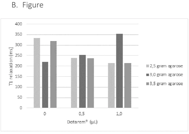
The T1 relaxation times of the samples mimicking bone are displayed in Figure 14. The T1 relaxation times mimicking muscle and fat are displayed in Appendix B (Figure 19, Figure 20). The calculated T1 relaxation times seem inconsistent. Although we expected the T1 relaxation times to lower as Dotarem® concentrations increased, we only saw this effect at concentrations of 1.0, 1.2 and 2.5 gram agarose. In all samples with higher agarose concentrations the T1 relaxation times were inconsistent.

The calculated T1 relaxation times of the bone and fat samples are higher than the calculated T1 relaxation times of the bone and fat tissue of the human knee, while the T1 relaxation times of the muscle samples are lower than the T1 relaxation time of muscle tissue.

The intensities of the T2 relaxation times of the samples mimicking bone, muscle and fat tissue are displayed in figure 16. The average R² of the intensity curve for the T2 calculation in the bone samples is 0.11 (0-0.3771), in the fat samples is 0.32 (0.1432-0.4519) and in muscle samples 0.35 (0-0.8273), which is very low. We do not make a calculation for the T2 relaxation time of the samples, due to low R² values.

(32)

32

FIGURE 16: INTENSITIES OF BONE, FAT AND MUSCLE SAMPLES VERSUS TE TIMES, USED TO CALCULATE T2 TIMES

Phase II Metal artefact research

II.B MRI measurements

In Figure 17 MR images of the healthy knee with TKA prosthesis and Figure 18 shows the MR images of the phantom with knee prosthesis. Both Figure 17A and Figure 18A are scanned with the FSE PD X- MAR sequence (metal artefact reducing) and both Figure 17B and Figure 18B with the FSE PD sequence/settings. In all 4 images a few metal artefacts are visible: a black haze at the place of the prosthesis and some bright white spots, probably caused by the prosthesis. It is clearly visible that the artefacts in surrounding structures next to the prosthesis show much larger artefacts in the human knee than in the phantom. In Figure 17B some metal splinters in the femur are visible.

[image:32.595.73.435.69.289.2]

(33)

33

FIGURE 17:A.FSEPDX-MAR;THICKNESS 4.0 MM,TR2560 MS,TE25 MS.B.THICKNESS 4.0 MM,TR2860 MS,TE 12 MS

FIGURE 18:A.FSEPDX-MAR;THICKNESS 4.0 MM,TR2560 MS,TE25 MS.B.THICKNESS 4.0 MM,TR2860 MS,TE 12 MS

II.C Examination of metal artefacts

(34)

34

TABLE 3:SIZE MEASUREMENTS ARTEFACTS PROTHESIS.*NM: NOT MEASURABLE, THE ARTEFACT SIZES ARE TOO LARGE TO MEASURE.**71++: THE ARTEFACTS EXCEED THE RANGE OF THE SLICES, SO THE HEIGHT IS AT LEAST 71. ***L,R:LEFT, RIGHT.“-“: PARAMETERS ARE NOT MEASURABLE IN THE CHOSEN IMAGING PLANE

Sequence Phantom/

participant Height (V+W+Z) Width (M/L) Anterior width (A/P - X - Y)

Posterior width (Y) Condyle (i-i) Condyle (c-c) Condyle (o-o)

Real size Participant 59.8 72 7 10 26 49 -

Phantom 54 71 5 7L, 4R*** 15 44 71

FSE PD X-MAR Participant 68 72 5 9 - - -

Phantom 83 88 20 13 - - -

FSE PD Participant 63 79 19 21 - - -

Phantom 70 88 9 15 - - -

Fast STIR X-MAR

Participant 71 59 - - 22 45 68

Phantom 71++** 72 30 25L,23R*** 27 48 82

Fast STIR Participant 92 77 - - NM* 72

Phantom 71++** 70 15 25 6 45 88

X-Bone Participant 61 76 - - 15 43 70

(35)

35

Discussion

The objective of this research is to investigate how a representative phantom can contribute to enhanced imaging of a TKA prosthesis in low-field MRI. First we will discuss if our self-made phantom is representative. Then we will comment on the accuracy of the analysis which conclusions can be drawn from this research.

Phase I material concentration research

I.A Preparation of material samples

The used method of heating the samples has some flaws. The samples were made in beakers with varying sizes and the temperature of the heating plate differed throughout the preparation of the samples. Both influence the speed of the heating process. A previous research set-up that aimed to produce accurate samples established that the use of an oil bath in combination with a porcelain container is a better method to heat the samples. [33] In other studies a water bath is used for heating the samples, following by heating in a microwave. [12] However, in this research it was not possible to use this kind of equipment. This might have resulted in more foam and different viscosities in the samples. Because the samples scorched very quickly at high temperatures, the samples were heated until 95 degrees, which is slightly below the maximum range of 90-100 degrees Celsius in which agarose dissolves. This could have influenced the homogeneity of the samples and makes the samples less comparable.

Prolonged heating can cause the gelatine to degrade. In this research the samples have not been heated for more than 30 minutes so a maximum of 6% decrease in gel strength has occurred. When the samples are heated for a longer period of time this decrease in strength should be taken into account. [42] Dotarem® was added with a pipet that was not accurate enough for the weighted amount. Since this amount is very small, a tiny variation could have influenced the T1 time considerably. In previous studies corrections were made for the evaporated water that was lost during heating. [33] In our research the samples were heated a lot shorter and the weight of the sample was not influenced because the sample was made out of a proportion of the total heated sample.

I.B MRI measurements

(36)

36 Figure 11 shows a few artefacts. The images show a dark line from top to bottom in the middle. The background changes from black to grey to white on the side of the images with a TE of 80, 90, 100, 110 and 120ms. This is a RF overflow artefact, which occurs when the measured signal exceeds the dynamic range of the analog-to-digital converter. As both the background and the samples change in intensities the measured values are less accurate. [21,22]

A lot of the samples show parallel lines at the sample boundaries and in some knee tissue parallel lines are visible as well. These are truncation artefacts which occur when the image contains high-contrast boundaries. This causes the samples to be less homogenous and thus influences the measured intensities. [31] A clear example can be seen in Figure 12 in the intensities of the large gelatine sample.

In the T2 images with a TE of 90 and 100ms chemical shift artefacts were visible around the edges of the samples. [29] This is not really a problem since the measurements are done in the centre of the samples.

I.C Examination of relaxation times

To calculate the T2 relaxation time, a decreasing exponential curve of the sample intensities at increasing TEs is needed. Some of the measured intensities of the samples are increasing instead of decreasing at increasing TEs. When this is the case the R² value of the intensity curve is close to zero. The R² values of the bone, muscle and fat mimicking samples are respectively 0.11, 0.32 and 0.35. The cause of the increasing sample intensities lies in corrupted images. The images with TE times above 80ms seem corrupted (Figure 11) The background (air) of these images has a bright colour which indicates a low SNR. After correction for the background intensity some values of the sample intensities became negative. These negative values occur as the background had a higher intensity than some of the samples.

The ROIs drawn in MATLAB R2016a where selected individually. Therefore it is possible that in some calculations a proportion of the sample container was included, which results in wrong intensity values. With the used MATLAB script however it was not possible to do this differently. Ikemoto at al. had set their ROI at a standard diameter. [13] In this way the measured pixels are the same for every sample, which results in a more reliable comparison between samples.

The predicted curve, plotted with the function fit in MATLAB R2016a, changes a lot by one of more extreme intensity values. This has an influence on the calculated relaxation times and on the R² of those values as well. The mean R² for the T2 values of the healthy knee is 0.67 (0.4816-0.8760).

Phase II Metal artefact research

II.A Preparation of phantom with prosthesis

In the creation of a phantom with a prosthesis, the idea is to place the prosthesis in the phantom in the same position as the prosthesis in the human knee. Unfortunately, the position of the prostheses in the phantom and the human knee did not correspond exactly. The position of a metallic implant in a MRI scanner, matters for the size of the artefacts as well as the position of the participant or phantom. [38] As the position of prostheses is different, a comparison between the artefacts in the phantom with prosthesis and the human knee with prosthesis is less reliable.

(37)

37 the images of the phantom with prosthesis and the artefacts in the images of the human knee with prosthesis is not reliable.

II.B MRI measurements

When comparing the images of the phantom with prosthesis and the human knee with prosthesis some striking results show up. Both images of the normal FSE sequence show more detail in surrounding structures than the X-MAR sequence, but in the images of the phantom with prosthesis the metal artefacts are larger with the X-MAR sequence. This is strange because the X-MAR sequence is specifically made to reduce metal artefacts. The metal artefacts in the X-MAR image of the human knee with TKA prosthesis are however reduced. The results are confusing, because they are conflicting. It may be possible that some data is corrupt and caused a reversal of the images of the phantom with prosthesis. The image that seems to be a FSE PD X-MAR is in real the standard FSE PD.

It is clearly visible that the artefacts in surrounding structures next to the prosthesis show much larger artefacts in the human knee with prosthesis than in the phantom with prosthesis. This result is remarkable and a reason could be that the phantom does not have these complex structures.

II.C Examination of metal artefacts

(38)

(39)

39

Recommendations

In order to make a more representative phantom for the enhanced imaging of patients with metallic knee implants, these are our recommendations for further research.

Sample preparation

In order to make the samples more consistent and reliable, it is recommended for future studies to change the process of sample preparation. The samples have to be made with more precision, using a more complex heating procedure with a two-step heating process. Using a hot oil or water bath to heat the samples will cause a more homogenate heating of the samples. [12,13,33]

Sample ingredients

When sample preparation techniques do not give the desired results, it is an option to use other T1 and T2 modifiers like Aluminium powder or Copper ions. Another option is to change the gelling agent to carrageenan. This gelling agent worked for other studies. [12,13]

Retrospectivity

In order to make the phantom as representative as possible, it should have the same structures and T1 and T2 values as human tissue. We expect that only when the phantom is representative, the artefacts can be fully compared. Making a more representative phantom is possible by making differences in density of the tissues (bone is hard, fat is soft). Another option in order to make the phantom more accurate is using a full TKA implant and not only a femoral part.

MRI

The MRI homogeneity can possibly be improved by redoing the calibration of the MRI scanner. If this has no effect, a calibration model that corrects for the attenuation at different locations in the coil should be made for the used parameters.

Sequences

Although the used spin echo sequence is able to calculate T1 and T2 relaxation times, newly created scans have made a lot of improvements. For example a Modified Look-Locker Inversion Recovery (MOLLI) sequence used for T1 mapping is a lot faster in calculating T1 relaxation times, but IR sequences can also be used for T1 and T2 calculation. [43] Therefore it will be wise to make an good evaluation before choosing a sequence.

Prostheses orientation

Susceptibility artefacts are greatly affected by the way metal is orientated with respect to the B0 field.

[44] When implant screws are orientated parallel to the B0 field, artefact sizes are minimal. In further

research it would be wise to think about the prostheses orientation in the B0 field.

Metal artefact examination

(40)

(41)

41

Conclusion

The phantom we created of gelatine, Dotarem®, agarose and demineralised water in this research is not representative for human tissue in low-field MRI. The T1 and T2 modifiers, Dotarem ® and agarose do influence the T1 and T2 relaxation times.

The phantom with prosthesis and the human knee with prosthesis do not show corresponding metal artefacts in low-field MRI in the used sequences. Out of the comparison of the phantom with prosthesis and the human knee with prosthesis it appears that complex structures are necessary for getting the same distortion.

(42)

(43)

43

References

[1] G.A. Poos MJJC, Hoe vaak komt artrose voor en hoeveel mensen sterven eraan, RIVM. (2014). [2] Datakwaliteit van de LROI, in: Orthop. Implant. Beeld, 2014: p. 116.

[3] OCON, Halve en hele knieprothese, Informatiebrochure OCON. (2015).

https://www.ocon.nl/media/Brochures/Knie_TKP_V1-05.pdf (accessed April 26, 2016). [4] Drugwatch, Knee Replacement Surgery, Drugwatch. (2016).

https://www.drugwatch.com/knee-replacement/surgery/ (accessed May 2, 2016).

[5] U. Cottino, F. Rosso, A. Pastrone, F. Dettoni, R. Rossi, M. Bruzzone, Painful knee arthroplasty: current practice, Curr. Rev. Musculoskelet. Med. 8 (2015) 398–406. doi:10.1007/s12178-015-9296-5.

[6] K.R. Math, S.F. Zaidi, C. Petchprapa, S.F. Harwin, Imaging of Total Knee Arthroplasty, (n.d.). [7] M.-J. Lee, S. Kim, S.-A. Lee, H.-T. Song, Y.-M. Huh, D.-H. Kim, S.H. Han, J.-S. Suh, Overcoming

Artifacts from Metallic Orthopedic Implants at High-Field-Strength MR Imaging and Multi-detector CT, RadioGraphics. 27 (2007) 791–803. doi:10.1148/rg.273065087.

[8] M.F. Koff, P. Shah, H.G. Potter, Clinical Implementation of MRI of Joint Arthroplasty, Am. J. Roentgenol. 203 (2014) 154–161. doi:10.2214/AJR.13.11991.

[9] M. Thomsen, U. Schneider, S.J. Breusch, J. Hansmann, M. Freund, [Artefacts and

ferromagnetism dependent on different metal alloys in magnetic resonance imaging. An experimental study]., Der Orthopäde. 30 (2001) 540–4. doi:10.1007/s001320170063.

[10] T.J. Bachschmidt, R. Sutter, P.M. Jakob, C.W.A. Pfirrmann, M. Nittka, Knee implant imaging at 3 Tesla using high-bandwidth radiofrequency pulses., J. Magn. Reson. Imaging. 41 (2015) 1570–1580. doi:10.1002/jmri.24729.

[11] A. Hellerbach, V. Schuster, A. Jansen, J. Sommer, MRI Phantoms - Are There Alternatives to Agar?, PLoS One. 8 (2013).

[12] K. Yoshimura, H. Kato, M. Kuroda, A. Yoshida, K. Hanamoto, A. Tanaka, M. Tsunoda, S. Kanazawa, K. Shibuya, S. Kawasaki, Y. Hiraki, Development of a tissue-equivalent MRI phantom using carrageenan gel, Magn. Reson. Med. 50 (2003) 1011–1017.

doi:10.1002/mrm.10619.

[13] Y. Ikemoto, W. Takao, K. Yoshitomi, S. Ohno, T. Harimoto, S. Kanazawa, K. Shibuya, M. Kuroda, H. Kato, Development of a human-tissue-like phantom for 3.0-T MRI., Med. Phys. 38 (2011) 6336–42. doi:10.1118/1.3656077.

[14] G.P. Mazzara, R.W. Briggs, Z. Wu, B.G. Steinbach, Use of a modified polysaccharide gel in developing a realistic breast phantom for MRI, Magn. Reson. Imaging. 14 (1996) 639–648. doi:10.1016/0730-725X(96)00054-9.

[15] W.D. D’Souza, E.L. Madsen, O. Unal, K.K. Vigen, G.R. Frank, B.R. Thomadsen, Tissue mimicking materials for a multi-imaging modality prostate phantom., Med. Phys. 28 (2001) 688–700. doi:10.1118/1.1354998.

(44)

44

Phantom Using Carrageenan Gel, Magn. Reson. Med. 50 (2003) 1011–1017. doi:10.1002/mrm.10619.

[17] F. Keith L. Moore PhD, FIAC, FRSM, P. Anne M. R. Agur BSc (OT), MSc, Arthur F. Dalley PhD, Clinically Oriented Anatomy, 7th ed., Lippincott Williams & Wilkins, 2013.

[18] E.A. Makris, P. Hadidi, K.A. Athanasiou, The knee meniscus: Structureefunction,

pathophysiology, current repair techniques, and prospects for regeneration, Biomaterials. 32 (2011) 7411–7431. doi:10.1016/j.biomaterials.2011.06.037.

[19] OCON, Knie artrose (knieprothese), (n.d.). https://www.ocon.nl/patienten/aandoeningen-en-behandelingen/knie-artrose-knieprothese (accessed April 26, 2016).

[20] S.J. Fischer, J.R.H. Foran, Total Knee Replacement, OrthoInfo. (2015). http://orthoinfo.aaos.org/topic.cfm?topic=a00389.

[21] J.P. Ridgway, Cardiovascular magnetic resonance physics for clinicians: part I, J. Cardiovasc. Magn. Reson. 12 (2010) 71. doi:10.1186/1532-429X-12-71.

[22] E. Blink, MRI : Principes, (n.d.).

[23] T. Magee, M. Shapiro, D. Williams, Comparison of High-Field-Strength Versus Low-Field-Strength MRI of the Shoulder, Am. J. Roentgenol. 181 (2003) 1211–1215.

doi:10.2214/ajr.181.5.1811211.

[24] E.D. Elster, Advantages of Low-Field Scanners, Elster LCC. (2015).

http://mriquestions.com/advantages-to-low-field.html (accessed April 22, 2016).

[25] A. Boss, H. Graf, A. Berger, U.A. Lauer, H. Wojtczyk, C.D. Claussen, F. Schick, Tissue warming and regulatory responses induced by radio frequency energy deposition on a whole-body 3-Tesla magnetic resonance imager, J. Magn. Reson. Imaging. 26 (2007) 1334–1339.

doi:10.1002/jmri.21156.

[26] P.A. BOTTOMLEY, P.B. ROEMER, Homogeneous Tissue Model Estimates of RF Power Deposition in Human NMR Studies, Ann. N. Y. Acad. Sci. 649 (1992) 144–159. doi:10.1111/j.1749-6632.1992.tb49604.x.

[27] M.B. Weishaupt D., Köchli V.D., How does MRI work, Springer, 2003.

[28] P.M.R. McRobbie D.W., Moore E.A., Graves M.J., MRI from picture to proton, in: MRI from Pict. to Prot., Cambridge University Press, 2004.

[29] A.W.M. van der Graaf, P. Bhagirath, S. Ghoerbien, M.J.W. Götte, Cardiac magnetic resonance imaging: artefacts for clinicians., Neth. Heart J. 22 (2014) 542–9. doi:10.1007/s12471-014-0623-z.

[30] J.F. Schenck, The role of magnetic susceptibility in magnetic resonance imaging: MRI magnetic compatibility of the first and second kinds, Med. Phys. 23 (1996) 836–840.

[31] K. Krupa, M. Bekiesińska-Figatowska, Artifacts in magnetic resonance imaging., Pol. J. Radiol. 80 (2015) 93–106. doi:10.12659/PJR.892628.

[32] Saba L., Image Principles, Neck, and the Brain, Taylor & Francis Group, 2015.

(45)

45

[34] K.P. Whittall, A.L. MacKay, D.K.B. Li, Are mono-exponential fits to a few echoes sufficient to determine T2 relaxation for in vivo human brain?, Magn. Reson. Med. 41 (1999) 1255–1257. doi:10.1002/(SICI)1522-2594(199906)41:6<1255::AID-MRM23>3.0.CO;2-I.

[35] T.S. Curry, J.E. Dowdey, R.C. Murry, Christensen’s Physics of Diagnostic Radiology, Med. / Anthony B. Wolbarst Phys. Diagnostic Radiol. Phys. (1993).

[36] R.L. Ehman, M. Brant-Zawadzki, M. Brant-Zawadzki, Reproducibility of Ti and T2 Relaxation Times Calculated from Routine MR Imaging Sequences: Phantom Study Bent 0. Kjos1, (1984). [37] J. Zhuo, Rao, P. Gullapalli, AAPM/RSNA PHYSICS TUTORIAL AAPM/RSNA Physics Tutorial for

Residents MR Artifacts, Safety, and Quality Control 1, (n.d.). doi:10.1148/rg.261055134. [38] S. Heiland, From A as in Aliasing to Z as in Zipper: Artifacts in MRI, Clin Neuroradiol. 18 (2008)

25–36. doi:10.1007/s00062-008-8003-y.

[39] R. Sutter, R. Hodek, S.F. Fucentese, M. Nittka, C.W.A. Pfirrmann, Total knee arthroplasty MRI featuring slice-encoding for metal artifact correction: reduction of artifacts for STIR and proton density-weighted sequences., AJR. Am. J. Roentgenol. 201 (2013) 1315–1324. doi:10.2214/AJR.13.10531.

[40] Zimmer ® NexGen ® RH Knee Primary/Revision Zimmer NexGen RH Knee Primary/Revision Surgical Technique, (n.d.).

[41] K.P. Somasundaram K, Analysis of Imaging Artifacts in MR Brain Image, Orient. J. Comp. Sci. Technol. 5 (2012). http://www.computerscijournal.org/vol5no1/analysis-of-imaging-artifacts-in-mr-brain-images/.

[42] P. Leiner, Gelatin Handbook, 888 (2012) 455–3556. http://www.gelita.com (accessed June 20, 2016).

[43] S.A. Smith, R.A.E. Edden, J.A.D. Farrell, P.B. Barker, P.C.M. Van Zijl, Measurement of T1 and T2 in the cervical spinal cord at 3 tesla., Magn. Reson. Med. 60 (2008) 213–9.

doi:10.1002/mrm.21596.

[44] A. Guermazi, Y. Miaux, S. Zaim, C.G. Peterfy, D. White, H.K. Genant, Metallic artefacts in MR imaging: effects of main field orientation and strength., Clin. Radiol. 58 (2003) 322–8. http://www.ncbi.nlm.nih.gov/pubmed/12662956 (accessed June 16, 2016).

[45] T.J. Heyse, L.R. Chong, J. Davis, F. Boettner, S.B. Haas, H.G. Potter, MRI analysis of the component–bone interface after TKA, Knee. 19 (2012) 290–294.

(46)

(47)

47

Appendix

A. Tables

TABLE 4:SAMPLE COMPOSITIONS

Sample Gelatin Agarose Dotarem (µL) Water NaN3

Bone1 10 gram 1,2 gram 3,5 90 gram -

Bone2 10gram 1,2 gram 4,0 90 gram -

Bone4 10gram 1,4gram 3,5 90 gram -

Bone5 10gram 1,4gram 4,0 90 gram -

Muscle1 10gram 2,5 gram 0 90 gram -

Muscle2 10gram 2,5 gram 0,5 90 gram -

Muscle8 10 gram 3,5 gram 0,5 90 gram -

Muscle9 10 gram 3,5 gram 1 90 gram -

Fat 1 10 gram 2,0 gram 3,0 90 gram -

Fat 2 10 gram 2,0gram 3,5 90 gram -

Fat3 10 gram 2,0gram 4,0 90 gram -

Fat 10 10 gram 2,0 gram 3,0 90 gram 0,03 gram

Fat 11 10 gram 2,2 gram 3,5 90 gram 0,03 gram

(48)

48

B. Figure

FIGURE 19:T1 TIMES OF MUSCLE SAMPLES.THE AVERAGE R² FOR THESE SAMPLES IS 0.99(0.9619-0.9969).

[image:48.595.71.385.73.295.2] [image:48.595.71.378.325.514.2]

(49)

49

FIGURE 21:MR IMAGE OF PHANTOM WITH PROSTHESIS;A.FAST STIR X-MAR,B.MR IMAGE FAST STIR

(50)

50

FIGURE 23:A.X-BONE IMAGE OF THE PHANTOM WITH PROSTHESIS,B.X-BONE IMAGE OF THE HUMAN KNEE WITH PROSTHESIS

(51)

51

C. MATLAB scripts

T1 calculation

%aantalscans= size(scans.data{1,:});

clear all

close all

scans = readDataServerPACS

%% T1 calculation

nr_samples = 16; %amount of samples in this box + 1 area for background

analysis

slice= 1 ; % kiezen welke slice

plaatje= 5; %selecteren vanaf welke scan je roi wil tekenen

%een hele hoop variabelen aanmaken

aantalscans2= size(scans.data(1,:));

aantalscans= aantalscans2(1,2) ;%aantal scans uitrekenen voor lengte

loopjes

ROI_space=logical(zeros(256,256,nr_samples));

scan=scans.data{plaatje}; %selecteren scan

nr_TR = size(scan,1); %aantal plaatjes in scan

image_space=zeros(256,256,nr_TR); %matrix aanmaken voor plaatje

image_space(:,:,nr_TR)=scan(slice,:,:); %plaatje selecteren

image=image_space(:,:,nr_TR) ; figure,

imshow(image_space(:,:,nr_TR),[]) %show image

ROI_space(:,:,nr_samples)=roipoly; %maken van ROI in plaatje

ROI_space2(:,:,nr_samples)=roipoly; %selection of background

intensities(plaatje,1) = mean(image(ROI_space(:,:,nr_samples))); intensities(plaatje,2) = mean(image(ROI_space(:,:,nr_samples)))-mean(image(ROI_space2(:,:,nr_samples)));

i=1;

for i=1: aantalscans

scan=scans.data{i}; %selecteren scan

image_space(:,:,nr_TR)=scan(slice,:,:);%derdeplaatje selecteren

image=image_space(:,:,nr_TR);

TR(i)=scans.info{1,i}.RepetitionTime;

if (i >= 1) && (i < plaatje) %andere afbeeldingen geen roi maken

scan=scans.data{i};

TR(i)=scans.info{1,i}.RepetitionTime; image=image_space(:,:,nr_TR);

intensities(i,1) = mean(image(ROI_space(:,:,nr_samples))); intensities(i,2) = mean(image(ROI_space(:,:,nr_samples)))-mean(image(ROI_space2(:,:,nr_samples)));

i=i+1;

elseif i==plaatje;

%lalalal niks doen

i=i+1;

else (i > plaatje) && (i <= aantalscans); scan=scans.data{i};

TR(i)=scans.info{1,i}.RepetitionTime;

(52)

52

i=i+1 ; end

end

close all

figure,

intensities(:,3) = TR ;%voor TR

[y,I]=sort(intensities(:,3)); gesorteerd=intensities(I,:);

gesorteerd=[0 0 0;gesorteerd]; %met 0'en aan het begin

x=gesorteerd(:,3); y=gesorteerd(:,2);

%modelfunctie maken en plotten

%maxTE= max(x);

figure,

%rekenen aan de modelfunctie

s = fitoptions('Method','NonlinearLeastSquares',...

'Lower',[0, 2 ,-inf],...

'Upper',[inf,inf, inf],...

'Startpoint',[0 0 0]);

f = fittype('(a-a*exp(-(x/b)))+c ','options',s);

[model,betrauwbaarheid] = fit(x,y,f)

xmodel= 0:0.25 :1500;

ymodel= (model.a-model.a*exp(-(xmodel/model.b)))+model.c;

figure,

plot (xmodel,ymodel) hold on,

plot (x,y,'o')

xlabel('TR') %voor T1 -> TR

ylabel('Intensities (I)')

ymax=max(ymodel);

yt2=(1-(1/exp(1)))*(ymax); %63.2% of the curve

syms xmodel

(53)

53

T2 calculation

clear all

close all

scans = readDataServerPACS

%%

%% poging doen tot andere scripts lezen T2 %aantalscans= size(scans.data{1,:});

aantalscans= 10; %aangeven aantal plaatjes te analyseren(verschillende

TE/TR)

nr_samples = 2; %amount of samples in this box + 1 area for background

analysis nr_TR= 1; intensities=(zeros(nr_TR,nr_samples)); ROI_space=logical(zeros(256,256,nr_samples)); i=1;

for i=1: aantalscans

scan=scans.data{i}; %selecteren scan

nr_TR = size(scan,1); % aantal plaatjes in scan

image_space=zeros(256,256,nr_TR); %matrix aanmaken voor plaatje

image_space(:,:,1)=scan(1,:,:);%derdeplaatje selecteren

image=image_space(:,:,1);

TR(i)=scans.info{1,i}.RepetitionTime; TE(i)=scans.info{1,i}.EchoTime;

if i==1 %%selecteren afbeelding

figure,

imshow(image_space(:,:,1),[]) %laten zien van de afbeelding

ROI_space(:,:,nr_samples)=roipoly; %maken van ROI in plaatje

%ROI_space2(:,:,nr_samples)=roipoly;

i=i+1;

elseif (i >= 2) && (i <= 5) %andere afbeeldingen geen roi maken

i=i+1;

else (i >= 6) && (i <= aantalscans);

intensities(i,2) = mean(image(ROI_space(:,:,nr_samples))); intensities(i,1) = mean(image(ROI_space(:,:,nr_samples)))-mean(image(ROI_space2(:,:,nr_samples))); i=i+1; end end

close all

figure,

(54)

54

intensities(:,3) = TE; %voor TE

[y,I]=sort(intensities(:,3)); gesorteerd=intensities(I,:); x=gesorteerd(:,3);

y=gesorteerd(:,1);

xlabel('TE') %voor T1 -> TR

ylabel('Intensities (I)')

%rekenen aan de modelfunctie

s = fitoptions('Method','NonlinearLeastSquares',...

'Lower',[100, -inf ],...

'Upper',[Inf,0],...

'Startpoint',[1 1]);

f = fittype('(a*exp((x*b))) ','options',s);

[model,betrauwbaarheid] = fit(x,y,f)

xmodel= 0:0.25 :150;

ymodel= (model.a*exp(xmodel*model.b)); x0= 0;

yt2= (model.a*exp(x0*model.b)) xt2= 0.368*yt2

figure,

plot (xmodel,ymodel) hold on

plot (x,y,'o')

ylabel('test')

syms xmodel

Enhanced imaging of metallic knee prostheses by using a representative phantom