1
Faculty of Electrical Engineering,
Mathematics & Computer Science
A rating model for individual player qualities
based on team results, applied in football
Anatolij I. Babiˇc
MSc Thesis
December 2017
Supervisors:
Preface
Before you lies the master thesis “A rating model for individual player qualities based on team re-sults, applied in football”. It has been written to fulfill the graduation requirements of the Applied Mathematics Master’s program at the University of Twente, Enschede. The project was undertaken in collaboration with SciSports, a football analytics company that is a spinoff from the University of Twente. From March to December, 2017, I have worked on this project, mostly from the SciSports office in Amersfoort and an improvised home office in Amsterdam. The research was very challenging and I’m happy to say that this work resulted in a novel method for player quality estimation in a multi-player environment.
I would like to thank my supervisors for their contributions and in-depth inspiring discussions re-garding this research. Although Richard is not a huge football fan, I’m very happy with his excellent support and advice during this project. I would also like to thank Jan for sharing his expertise regarding the formulation of ideas that resulted in the eventual model.
I hope you will read this thesis with great interest.
Anatoliy Babic
Abstract
There are abundant situations where teams of players compete. The competing players have qual-ities that influence the outcome of a match, but in some cases, individual contributions are not recorded and only team results can be observed. Examples can be found in sports (football, basket-ball, volleybasket-ball, etc.), e-sports (Dota, StarCraft, League of Legends, etc.), film-making and company management. In this research, we developed an individual player quality inference algorithm which only requires historical team results. Whenever groups of individuals produce collective results and we do not have the data regarding individual contributions, our model can be applied.
Most existing models that are used to estimate individual qualities deal with 1-vs-1 matches, with a single quality per player and a single binary outcome per match. Our model is an extension of existing models; providing a structure to deal with multiple individual qualities, for many-vs-many matches and multiple outcomes per match, each with an ordinal outcome space. The goal was to create a model for any environment where groups of players compete with each other while only the collective results are observed. The research was conducted in partnership with SciSports, a football data analytics company, therefore we chose to apply the model to football.
We considered multiple existing models like ELO, Glicko, Bradley-Terry, Thurstone-Mosteller and the Microsoft TrueSkill. We combined ideas from these models with novel insights to define a probability model, defining the relationship between participating player’s qualities and the match-outcome dis-tribution. This relationship is essential for the inference of player quality parameters. The unknown parameters that define the player specific qualities are modeled as latent traits within a latent variable model. We started with a general model, developed in the field of psychometrics, and showed that it is equivalent to our desired model under certain assumptions. Furthermore, we discuss how ordinal observations should be interpreted and we find accurate and useful approximations for the ordinal outcome probability distribution given player participation.
We list several existing estimation methods that can be used to extract estimators from the data by applying our probability model. The methods were taken from other research and modified such that they can be applied to our specific case.
Contents
1 Introduction 1
1.1 Player quality estimation . . . 1
1.2 Existing models . . . 1
1.3 Our approach . . . 2
1.4 Contributions . . . 2
2 Literature study 3 2.1 Strategy benchmarking . . . 3
2.2 Statistical player metrics . . . 4
2.2.1 Plus-minus statistic in basketball and ice-hockey . . . 4
2.3 Pairwise comparisons . . . 5
2.3.1 Bradley-Terry model . . . 5
2.3.2 Thurstone-Mosteller model . . . 6
2.4 Pairwise comparison models with non-binary outcomes . . . 6
2.5 Rating models . . . 7
2.5.1 ELO-rating . . . 8
2.5.2 Glicko-rating . . . 8
2.5.3 Dutch tennis league rating system . . . 9
2.6 Microsoft TrueSkill . . . 10
2.6.1 Model . . . 10
2.6.2 Model performance . . . 11
2.7 Coalition Assessment in Film-Making . . . 11
3 Mathematical model 13 4 Probability model 18 4.1 Relationship between KPI outcomes and strength difference . . . 18
4.2 IRT model . . . 19
4.2.1 Strength difference utility function . . . 20
4.2.2 Benchmark parameter estimation . . . 21
4.2.3 Improved benchmark parameter estimation . . . 21
4.2.4 Gaussian distribution as link function . . . 22
4.3 Observed strength difference . . . 23
4.4 Market knowledge . . . 24
5 Estimators for mean quality, quality variance and player inconsistency 26 5.1 Maximum likelihood estimation . . . 27
5.2 Ordinary least squares . . . 28
5.3 Generalized least squares . . . 30
5.4 Regularized estimates . . . 30
5.5 Batch inference . . . 31
5.5.1 Woodbury matrix identity . . . 32
5.6 Conditional Gaussian inference . . . 32
5.6.1 Batch processing . . . 33
5.7 Estimation using bookmaker predictions . . . 34
5.7.1 Bookmaker maximum likelihood . . . 35
5.7.2 Bookmaker implied strength difference . . . 35
5.8 Dynamic player qualities . . . 35
5.9 Discussion of methods . . . 36
6 Results 37 6.1 Model parameters . . . 37
6.1.1 Implementation Specifics . . . 38
6.2 Player ranking . . . 39
6.3 Match outcome prediction . . . 41
7 Conclusions and recommendations 43 7.1 Assumptions and shortcomings . . . 43
8 Table with variable definitions 45
A KPI outcome probability model 46
A.1 Intuitive explanation of methodology . . . 46
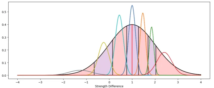
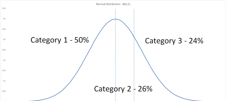
A.1.1 Visualisation of Gaussian distribution as a link function . . . 46
A.1.2 Applicability to Poisson distribution . . . 47
A.2 Bayesian two-dimensional rating inference . . . 48
B Estimators 50 B.1 Bias-variance decomposition . . . 50
B.2 Minimum mean squared error . . . 50
C Gaussian random variables 51 C.1 Truncated Gaussian distribution . . . 51
C.2 Multiplication of Gaussian PDFs . . . 51
C.3 Multivariate Gaussian distribution with multivariate Gaussian mean . . . 51
C.4 Marginal Gaussian inference equations . . . 52
C.5 Convergence and asymptotic unbiasedness of conditional Gaussian . . . 52
C.6 Bayesian Inference of a Multivariate Normal Distribution . . . 54
C.7 Application of Bayesian Inference with unknown partial observations . . . 54
D Heteroskedastic player inconsistency 57 D.1 Heteroskedasticity - maximum likelihood estimation . . . 58
D.2 Heteroskedasticity - least squares . . . 58
D.3 Heteroskedasticity - p-norm difference . . . 59
D.4 Heteroskedasticity - relative error . . . 59
D.5 Heteroskedasticity - almost unbiased estimator . . . 60
[image:5.595.95.515.59.396.2]1
Introduction
There are abundant situations in reality where a coalition of players collaborate to achieve a collective set of goals. Such players have certain skills that often cannot be measured directly, but are an explanatory variable for historical and future results. The goal of this research is to find an algorithm that estimates individual player skill quality by using historical results achieved by coalitions of players. We do this by modeling the relationship between quality, performance and realized outcome and applying estimation techniques to infer player quality from historical results.
Some examples of collaborating teams with collective observable outcomes are start-up company entrepreneurs, football players and film-making teams. In film-making, a team of professionals works together to produce a profitable and qualitative end product. In a start-up company, a small team of entrepreneurs and professionals collaborate to build a profitable business. In the game of football two teams compete with the objective to score more often than their opponent. In these environments, it is possible to observe collective results, but there is a need to understand contributions of individuals to the achievements of a team. Individual achievements are often difficult to extract because of the collaborative nature of the environment. Most individual results are (partly) a team performance, rather than purely an individual performance.
1.1
Player quality estimation
Knowledge regarding player qualities can be very useful for decision-making purposes. Numerical evaluations of the qualities of film-makers can be used in the decision-making progress of funding al-location for future films (Timmeret al., 2017). Whenever playing online on the Xbox, the opponents are done by a match-making system that uses player quality estimates to pair evenly matched players, hereby avoiding that an advanced player will play against players that are new to the game (Herbrich
et al. , 2007). Accurate player quality estimates provide an understanding of hidden variables that can be used to explain historical and predict future performances.
In game theory, the importance of individual contributions to coalitions has been extensively re-searched. Coalitions have a value, which can be distributed over the coalition members in according to certain criteria. The Shapley value is a uniquevalue distributionthat follows from a set of desirable properties. The Core is a set of value distributions that cannot be improved upon by sub-coalitions (Gillies, 1959).
A different approach to estimating player quality, is by benchmarking a player’s strategy tothe op-timal strategy. Another approach would be to perform cognitive or physical tests and use the results as a proxy for player quality.
Our research focused on environments where wedo not have observations of individual performances of players. Our approach is data-driven; the only input required is data of match outcomes and player participation. Our model requires a very limited amount of domain knowledge; i.e. what we require from domain experts are weights that assign importance to qualities in certain situations. Wedo not
need to model the game environment, understand successful strategies or know the exact rules.
1.2
Existing models
There are existing models that assign a value to player qualities.
In game theory, the value of individual contributions in coalition games is a very important result. Whenever the values of all sub-coalitions are known the value of individuals within a game can be characterized by the Shapley value (Shapley, 1953).
In some environments, we can have a round-robin tournament (all-play-all) schedule and yield a ranking for all the players. The main disadvantage of this is the large amount of (possibly irrelevant) matches that need to be played. A different approach is to keep track of player qualities in a so-called
rating system. A rating system keeps track of player ratings, can predict the outcome probability from the ratings of player and updates the ratings after every encounter. Ideally, such a rating is a representation of skill.
method. It models the player quality as a Gaussian random variable. This improved the error and convergence of the ratings. The Microsoft TrueSkill algorithm (Herbrich et al. , 2007) model is designed for multi-player environments, applying state-of-the-art modeling techniques (factor graphs) and inference algorithms (Expectation Propagation).
Player qualities can also be estimated with statistical approaches. The plus-minus method applies linear regression between player participation and outcomes (Fitzpatrick, 2017; Rosenbaum, 2004). The qualities of film-makers can be estimated by a linear estimator using the success of films made in the past (Timmeret al., 2017).
Another existing individual player rating model has been developed by SciSports, the company for which we performed this research. The model is called SciSkill, was developed especially for football and covers more than 70.000 football players from the whole world. It is a difference based approach inspired by the ELO rating system. The algorithm contains a lot of components that solve problems in a very pragmatic way. The model was built with a focus on application, therefore certain parts of the algorithm lack scientific justification. The model is not published, and therefore we will not discuss it in the literature study.
1.3
Our approach
Our focus is finding a method to estimate player qualities, without using any individual data, only team results. We assume that player quality, an unobservable variable, has a stochastic relationship with historical outcomes and future outcomes. The historical outcomes can be used to estimate the qualities, and the estimates we yield can be used for prediction of future matches. We assume the player quality to be non-deterministic, therefore it is modeled as a random variable. As players perform in teams, against other teams, we require a way to aggregate performances. We assume that a useful aggregation can be achieved by a weighted sum of the individual qualities. This aggregation has a non-linear relationship with the observed outcomes. We define this relationship with a probability model.
After the construction of the probability model, we apply estimation techniques that extract player quality parameter from the historical data. The estimation techniques use different assumptions and optimization criteria. The estimators we find are tested according to a subjective criterion (player rankings) and an objective criterion (future match prediction).
Due to the assumptions and modeling choices, the abstract problem we solve in this research is parameter estimation of a normal distributions, if we only observe a specific non-linear transformation of an affine transformation of the realizations of this normal distribution.
1.4
Contributions
2
Literature study
There have been efforts to create effective algorithms that infer the qualities of individuals. Such qualities are latent variables, as they cannot be observed directly, but have a relationship with ob-servable quantities. Therefore accurate quality models can be used to analyze historical outcomes and predict future outcomes.
The first type of quality estimation method we discuss is strategy benchmarking. The idea of this method is to assess the quality of players, by benchmarking their strategy to the optimal strategy. We discuss this approach in Subsection 2.1.
There are other methods that generate statistical metrics to assess player qualities. Such metrics are based on smart counting of past performances, which often misses out on a lot of context information. We discuss some of these statistical metric methods in Subsection 2.2.
Rating systems include a very important contextual element; the quality of the opponent is taken into account. Rating systems produce estimates of player ratings (unobservable latent variables), that are a representation of player quality. Rating systems use historical data to infer estimates of player ratings. Some possible data sources are polls, betting odds or historical results. A very important building block of a rating system is quality inference based on historical comparisons of two objects. Such experiments are called pairwise comparisons, and we describe methods that use these in Subsection 2.3. The outcomes of pairwise comparisons are traditionally binary, but in real-ity, outcomes often are ordinal or continuous. The most famous pairwise comparison models are the Thurstone-Mosteller and Bradley-Terry models, discussed in 2.3.2 and 2.3.1. We will discuss some extensions of the Bradley-Terry model that allows for draws in Subsection 2.4. We will continue with discussing rating systems in Section 2.5. The most famous rating systems are ELO and Glicko, these will be elaborated in 2.5.1 and 2.5.2 respectively.
A relatively new approach is the TrueSkilltm developed by Microsoft Research, specifically to achieve fair matchmaking for online games on the Xbox, Microsoft’s online gaming platform. The TrueSkill methodology applies Bayesian graphical modeling to infer player rating distributions from past re-sults, we discuss it separately in Subsection 2.6. Lastly, we discuss a coalition assessment model, that has been applied successfully to estimate the qualities of film-makers in Subsection 2.7.
Throughout this section, we will require the definition of likelihood L of parameters given a set of observations. Whenever we have parametersθand dataD, we define the likelihood of the estimator ˆ
θof the parameters θas:
Lθ= ˆθ;D=d=Pθˆ(D=d) (1)
Here we use the notation Pθˆ(D=d), which is the probability thatD =d under the condition that the parameterθ= ˆθ. The estimator ofθ that maximizes the likelihood, is defined as the Maximum Likelihood Estimator (MLE):
ˆ
θM LE = argmax ˆ θ
Pθˆ(D=d) (2) = argmax
ˆ θ
H Pθˆ(D=d) (3)
HereH : [0,1]→Rmust be a strictly increasing function.
2.1
Strategy benchmarking
The idea of this approach is to perform player quality estimation by evaluating the strategy (all decisions and actions) of a player with respect tothe game theoretical optimal strategy. Finding such an optimal strategy is very complex, but for our purposes, a strategy that can beat top human players is enough and evaluate game-states. The main assumption is that players with a high quality have a superior strategy over players with a high quality.
on reinforcement learning techniques explicitly have an internal game-state evaluation model, which makes it possible to evaluate all the decisions and actions given a certain game-state. This evaluation could be performed on past performance of individuals. A good example of such a method is the
centipawn loss system developed in chess, which calculates how much centipawns (1001 of a pawn) a player loses on average compared tothe computer move. A low centipawn loss can be seen as a good proxy for player quality. A nice feature of the centipawn methodology is that it has a dimension (centipawns lost per move), and therefore can be interpreted intuitively.
Due to increased computing power and the utilization of machine learning techniques, progress in the field ofsolving games has been: examples are Jeopardy (general knowledge quiz), Go (deterministic board game) and No-Limit Texas Hold’em (stochastic card game).
Remark 1. Some games are not solved due to the fact that not only decisions need to be made, but they also need to be executed with precision. Examples of such games are football, golf, ping-pong, Dota 2 and StarCraft. In football, Robocup is an ongoing initiative, started in 1997 (Robocup, 2017), with the ambitious goal of designing humanoid robots to beat real humans at football before the year 2050 (Kitano et al., 1997). There has been research with the goal of designing robots that can autonomously play ping-pong (Peterset al. , 2013). Very recently, the company OpenAI successfully developed a bot for 1-vs-1 matches in the game Dota 2, beating top human players (OpenAI, 2017).
We expect more games to be solved by algorithms in the future. We expect rating systems based on the described approach to be very accurate. An assumption of this approach is that an optimal strategy in human vs human matches is equal (or at least similar) to the strategy a computer chooses. Unfortunately, this is not always true; psychological mind-games and intimidation can play a big role in human-vs-human matches, while a computer algorithm would never be influenced by this. An important quality in human-vs-human matches is to understand your opponents (weaknesses and strengths), while thisquality is irrelevant against a strictly better computer algorithm and therefore will not be measured.
2.2
Statistical player metrics
There are models that focus on finding statistical metrics to quantify player performance. In the sport of football examples are: goals scored, successful pass percentage and expected goals. All these metrics are a weighted counting technique, where often context is not fully captured. Goals scored can, for example, be skewed because a player played a lot, or because a player takes penalties. It is always interesting to normalize quantities (apply relevant dimensions), e.g. non-penalty goals per 90 minutes played instead of total goals. A nice property of such methods is that statistical assessments (metrics) have a dimension, which often allows for intuitive interpretation and usage. The plus-minus statistic is a more elaborate statistical method, discussed in detail in Section 2.2.1.
In (Tiedemann et al. , 2011) the performance of players is evaluated based on a non-parametric concave meta-frontier approach. The meta-frontier defines a theoretical optimal player performance, based on the playing time and position of the best player. This permits estimation of all players’ efficiency. A positive correlation has been found between players’ efficiency and their historical team performance. We believe the main reason for this relationship is that (within this method) goals for and goals against form a very important factor in determining the efficiency of players and success of teams. The method does not provide any predictive capabilities.
A data-driven method to determine the ability of soccer players entirely based on the value of their completed passes was developed by (Brookset al., 2016). Passes are valued according to location and shot opportunities generated. The relationships are learned from data and mostly work for offensively minded players.
2.2.1 Plus-minus statistic in basketball and ice-hockey
The plus-minus statistic (PM) is a statistical measure to determine the average added value of basket-ball players in the NBA (Rosenbaum, 2004) and NHL (Fitzpatrick, 2017). The simplest interpretation of this rating system is a virtual counter of the total goals a team scores minus the total goals a team concedes, whenever a player is in the field. The system looks at player participation, and sets up a linear system for each part of the match where there is no substitution:
Only players that reach a minimum amount of minutes receive a personal rating, other players are grouped in the variableq0. Lastly;δi = 1, if playeriplays for the home team, andδi=−1 if a player plays for the away team. The plus-minus statistic is very dependent on the context wherein a player performs, mostly the quality of his own team and the opponents team. Because of the lack of context incorporated in the plus-minus calculation is biased and a player with the exact same skill can get a different rating.
The plus-minus statistic can be extended to the adjusted plus-minus (APM) statistic, by separating the single equation for each match into two equations. This separation is done on a player level; yielding an equation for the time a player was in the field, and the other equation for the time this player was not in the field. The performance (realized score margin) of a team during the part of the match when the player is in the field and when he is on the bench are compared. This way we can detect differences in performance of a team whenever a single player is playing. By using this approach we eliminate the influence of own team strength and opponent strength.
One of the main requirements for using PM is a high scoring frequency. Furthermore, the APM approach works optimally in sports where a line-up is constantly changing during the game.
2.3
Pairwise comparisons
In this section, we will call the players/objects that are compared pi, and they will have a quality rating ofqi. The rating of all players is represented in the vectorq. Depending on the model, player qualities are defined as a parameter or a random variable. In the case that the qualities are random variables, we takeqi ∼Qi. We call the variableDij the outcome of the pairwise comparison ofiand
j and define it such that:
Dij =
1 ifiwins 0 ifj wins
1
2 idrawsj
(5)
It holds that Dij+Dji = 1. In general, i and j could be compared multiple times, but we do not account for this in our notation.
There has been some fundamental research into pairwise comparisons. Two of the most used models in literature are the Bradley-Terry (Bradley & Terry, 1952) and Thurstone-Mosteller (Thurstone, 1927), (Mosteller, 1951) rating systems. Both approaches are not developed explicitly to deal with draws or multiple players, but the models can be extended to allow for such cases. We will discuss some examples of extensions in Section 2.4.
2.3.1 Bradley-Terry model
The Bradley-Terry approach (Bradley & Terry, 1952) considers that all the objects which are being compared have a constant rating parameter. In the original approach pairwise comparison experi-ments are considered with a binary outcome, not allowing for draws, with probabilities defined as:
Pq(Dij= 1) =
q1
q1+q2
= 1−Pq(Dij = 0) (6)
Parameters of teams can be estimated efficiently, multiple methods have been developed to achieve this. One method is a recursive Minorization-Maximization procedure (Hunter, 2004) applied to the log-likelihood function of observations. We define all our results as D, and calculate the probability of observing the resultsd, we can extractwij as the number of timesi has beatenj to get:
Pq(D=d) =
Y
i,j
q
i
qi+qj
wij
(7)
logPq(D=d) =X i,j
wijlog(qi)−wijlog (qi+qj) (8)
The maximum likelihood estimators for the parameters can be found with a method similar to logistic regression. A feasible solution exists under the condition that there is no partition of the players in two groups, where the outcomes of all comparisons between players from different groups have one-sided outcomes. If such a partition, of the whole player setP, were to exists, say pandpc so that
from pandpC) we require∃
i,ji∈p∧j ∈pc (wij >0). Under the previous scenario, our maximum likelihood solution will become:
ˆ
qBT−M LE = argmax q
(logPq(D=d)) (9)
ˆ
qBTi −M LE → ∞ ∀i, i∈p (10) ˆ
qBTj −M LE → −∞ ∀j, j∈pC (11) The values we calculate will diverge, which is a useless answer for our problem. This problem may occur when we have a small dataset and results between two groups are very one-sided, but fortunately it can be avoided by regularizing the player rating parameters. This can be done, according to a Bayesian approach by taking a prior distribution over the ratings q ∼ Q. We are left with the following log-likelihood to be maximized:
pD,Q(d, q) =P(D=d|Q=q)pQ(q) (12) log(pD,Q(d, q)) = log(P(D=d|Q=q)) + log(pQ(q)) (13)
ˆ
qBBT−M LE = argmax q
[log(P(D=d|Q=q)) + log(pQ(q))] (14)
2.3.2 Thurstone-Mosteller model
The Thurstone-Mosteller model (Thurstone, 1927) assumes that player ratings are random variables with a normal distribution, thus qi ∼ N(µi, σi2). In general, σi2 is player dependent, but often for simplicity it is chosen the same for all players. The model now states that the winner of a paired comparison is the player with the highest player performance, which has the same distribution as his rating. We get the following:
P Dij = 1|qi∼ N(µi, σi2), qj ∼ N(µj, σj2)
=P qi> qj|qi∼ N(µi, σi2), qj ∼ N(µj, σj2)
=P X >0|X ∼ N(µi−µj, σ2i +σ2j)
= 1−P X <0|X ∼ N(µi−µj, σ2i +σ 2 j)
= 1−Φ
µj−µi
q
σ2 i +σ
2 j
= Φ
µi−µj
q
σ2 i +σj2
Here we use that Φ is the standard normal cumulative distribution function. This shows that the Thurstone-Mosteller model is a linear probit model (Albert & Chib, 1993). The ratings can be estimated efficiently by assuming that the rating distributions are constant during the complete period during which the pairwise comparisons were performed. The complete likelihood function becomes:
q∼ N(µ,Σ) (15)
L(µ,Σ;D=d) =Pµ,Σ(D=d) (16)
=Y i,j
DijΦ
µi−µj
q
σ2 i +σj2
+ (1−Dij)
1−Φ
µi−µj
q
σ2 i +σj2
(17)
ˆ
µT M−M LE,ΣˆT M−M LE= argmax µ,Σ
[L(µ,Σ;D=d)] (18)
Gibbs sampling can be used to efficiently find the MLE for the above likelihood expression.
2.4
Pairwise comparison models with non-binary outcomes
extensions of the Bradley-Terry model with an outcome space ofN possibilities. A generalized Bradley-Terry model could look as follows;
P(Yij =k) =
ezk(i,j)
N
P
n=1
ezn(i,j)
(19)
Here the functionznis specific for outcomen, but depends on the participantsiandj. An extension of the Bradley-Terry approach by for the specific case of three outcomes, where two are decisive and one is non-decisive, a model was proposed by (Davidson, 1970):
P(Yij= 1) =
eqi eqi+eqj+eλ+12qi+
1 2qj
(20)
P
Yij = 1 2
= e
λ+1 2qi+12qj eqi+eqj+eλ+12qi+
1 2qj
(21)
P(Yij= 0) =
eqj
eqi+eqj+eλ+12qi+12qj
(22)
Another solution discussed in the same paper, the Rao-Kupper tie model, gives the following equa-tions:
P(Yij = 1) =
eqi
eqi+λeqj (23)
P(Yij = 1 2) = (λ
2−1) eqi+qj
(eqi+λeqj)(eqj+λeqi) (24) P(Yij = 0) =
eqj
λeqi+eqj (25)
where we require thatλ≥1. In the case thatλ= 1 reduces to the standard Bradley-Terry model. These two examples are both valid varieties of the generalized model described in Equation (19). We conclude that there is no single choice for the functions zn(i, j), and for specific applications, tailor-made solutions should be developed.
2.5
Rating models
In this subsection, we will discuss two rating models that are often used; ELO and Glicko. These models, as most rating models, use a latent variable that is a representation of player quality, and a mapping from the qualities of all players in a match to the match outcome. The main difference between the models is that ELO only estimates the first moment of player ratings, while Glicko also estimates the second moment. The probability model that is necessary for rating inference, can be used to predict future fixtures.
The main difference between previously discussed models and rating models, is that rating models incrementally process historical data. Therefore the produced ratings are a time series, showing the development of the rating rather than just a point estimate. Another attractive feature of rating systems is that they allow a continuous outcome space, as rating updates are performed as a function of difference between performance and expected performance. We use the following notation; qi is the prior and qnew
i is the posterior rating of player i. We define dSij as the prior rating difference and dSO
ij as the observed strength difference for a match between player i and j. Also, we need a monotonically increasing functiong(·) that gives us the update magnitude based on observed rating difference.
We get the following equations for the update after a match between playeri and playerj:
dSij =qi−qj =−dSji (26)
qnewi =qi+g(dSijO−dSij) (27)
2.5.1 ELO-rating
The ELO-rating is a widely used rating system, initially developed to determine the relative strengths of chess players, by applying an iterative inference process on game outcomes (Elo, 1978). The rela-tive strengths are parametrized as ratings, and can be used to generate match outcome probabilities for players that have never played each other.
The approach uses the Bradley-Terry paired comparison formula to determine match outcome proba-bilities. It applies a logarithmic transform on the ratings, using ˜qi=eqiwhere ˜qiare the Bradley-Terry strength parameters. We get the following relationship:
Eij =E[Yij] (29) = q˜i
˜
qi+ ˜qj
(30)
= e
qi
eqi+eqj (31)
= 1
1 +eqj−qi (32)
WhereEij corresponds to the average amount of points playerigets when competing against player
j, where a win counts for one point, draw counts as 12 point and a loss as zero points. We can observe that this implies that match outcome probabilities follow directly from the rating difference,qj−qi. The updating of ratings given a match outcome is done relative to the expected outcome, which is calculated with the player ratings. Whenever a player over-performs(under-performs) his rating will become higher(lower). This way the ratings slowly converge to their real value. In the ELO model the update equations look as follows:
qnewi =qi+K·(Yi−Ei) (33) WhereYi is the total points and Ei is the expected amount of points of playeri in the period since the last rating change. K is a parameter that determines the magnitude of the rating change. K is positive such that ratings of players increase (decrease) whenever players overperform (underperform). In general,K should be chosen higher for important matches. Friendly matches should have a lower
K factor, than a world cup final match. The choice of the K remains a domain and match specific problem. The system has received a lot of theoretical critique, and statistical improvements have been proposed by Glicko-model, discussed in the next subsection. Nonetheless the ELO-model remains the standard in a lot of disciplines. The main reason is that the ELO-model is much easier to understand, explain and implement than any other available alternative.
2.5.2 Glicko-rating
The Glicko-rating system (Glickman, 1999) was developed by Mark Glickman, it is an extension to the ELO-rating but it specifies the rating as a random variable. The rating of playerihas a normal distribution, we use the following notation:
Qi∼ N(µi, σi2) (34)
pQi(qi) =N(qi;µi, σ
2
i) (35)
the strength of the player under consideration andqk ∼Qkas the prior strength of hiskthopponent.
fQ(qi|D=d) =
Z
...
Z
fQi(qi|Q1=q1, ..., QN =qN, D=d)N(q1;µ1, σ
2
n)...N(qN;µn, σn2)dq1...dqN (36)
∝
Z
...
Z
N(qi;µi, σ2i)L(Qi=qi, Q1=q1, ..., QN =qN;D=d)N(q1;µ1, σ21)...N(qN;µN, σ2N)dq1...dqN (37)
=N(qi;µi, σi2) N
Y
j=1
Z
L(Q=q, Qj=qj;Di,j=di,j)N(qj;µj, σj2)dqj (38)
∝ N(qi;µi, σi2) N
Y
j=1
Z
P(Di,j=di,j|Q=q, Qj =qj)N(qj;µj, σ2j)dqj (39)
Here we use that N(x;µ, σ2) is the probability density function of a normal distribution with mean
µand variance σ2, evaluated in the pointx. In Equation (39) we use theDj ∈ {0,1}, which is the subset of D with the relevant data of outcomes of matches between player j and the player under consideration.
To proceed we need to have the outcome probability given the player ratings. Just like with ELO, as shown in equation (32), this is taken as a logistic distribution. Furthermore, the author uses an approximation from (Crooks, 2013) for the integral in Equation (39):
P(Di,j=Yi,j|Qi=qi, Qj=qj) =
(eqi−qj)Yij
1 +eqi−qj (40)
Z
P(Di,j=Yi,j|Qi =qi, Qj =qj)N(qj;µj, σ2j)dqj =
Z e(qi−qj)Yij
1 +e(qi−qj)N(qj;µj, σ
2
j)dqj (41)
≈
eg(σ2j)(qi−qj)
Yij
1 +eg(σ2j)(qi−qj)
(42)
g(σ2j) = 1
q
1 + 3σ 2
j
q2
(43)
Using this approximation, we yield the update equations for the rating of playeri:
µnewi =µi+ ( 1
σ2 i
+ 1
δi )−1
N
X
j=1 j6=i
g(σ2j)(Yij−E(Yij|µi, µj, σj2))
σinew= ( 1 σ2 i + 1 δ2 i
)−12
E[Yij|µi, µj, σj2] =
1
1 +e−g(σj2)(µi−µj)
δi2=
N X j=1 j6=i
g(σ2j)EYij
µi, µj, σ2j
(1−EYij
µi, µj, σ2j
) −1
The Glicko-system also describes a backward filtering step, using a Kalman Filter approach to extract improved estimators for previous time steps.
2.5.3 Dutch tennis league rating system
strength and uses the following formulae:
R(k)i =
qj−1 ifYij = 1 andqi> qj−1
removed ifYij = 1 andqi< qj−1
qj+ 1 ifYij = 0 andqi< qj+ 1
removed ifYij = 0 andqi> qj+ 1
(44)
qinew= 1
|M|
X
m∈M
R(m)i (45)
M ={Ri(k)|R(k)i 6=removed} (46) Here we have that M is a collection of matches that are not “removed” that were played during a certain year. During the start of each year, last year’s results are used to form the new player rating. The driving idea behind this rating system is that players are expected to win against an opponent with a rating that is one point higher (worse). Every player keeps a record of scored points; the score is relative to the opponent. Winning from a player means that your rating should be one less than his current rating, therefore your result record will contain this score. For players with large differences, more than one rating point, the expected outcome (lower rated player wins) will be classified as
removed. This means that a theoretical property of this rating is that players cannot improve their rating whenever they play against much lower rated players, but can worsen their rating (drastically). For this reason, it is very unattractive for competitive players that focus on getting a low rating to play against much weaker players.
There are manual, non-mathematical, adjustments to the model to deal with new players, player inactivity and infrequent playing results. The documentation explaining the system even contains a subsection elaborating that in some (extreme) cases the federation can manually adjust the ratings of players if there is a reason to do so. This shows that the federation employs the rating system as a guideline; adjusting where needed to ensure correctness in extreme cases.
2.6
Microsoft TrueSkill
The TrueSkill rating system (Herbrich et al., 2007) has been developed by Microsoft to be used in a broad spectrum of games offered on their Xbox game console. The main goal of this rating system is to match players with equivalent skills, in essence maximizing draw probability of matches. This way competitive matches between users on the platform ideally are between players of equal strength. TrueSkill is also suitable for multi-player games; it assumes that player qualities are additive. In the following sections, we will explain the model and discuss its performance.
2.6.1 Model
The model uses factor graphs to create a complete probability distribution of individual player skills, team skills, and game outcomes. The skill of individual i is modeled by the random vari-ableMi ∼ N(µMi, σ
2
Mi). Whenever a player performs, his performance isqi∼Qi=N(Mi, β), where β is a constant performance uncertainty for all players. Players perform in teams, and the team performances to be additive, thus:
Tj=
X
i∈Aj
Qi=N(
X
i∈Aj
Mi, β·NAj) (47)
NAj =|{i∈Aj}| (48)
Here Aj is the set of indices of players in coalitionj. The eventual ranking of the teams within a match is considered to be a direct consequence of the team performances, we define such ranking as
fed to the algorithm to produce improved beliefs of player quality parameters.
A very important part of the algorithm is the approximation method Expectation Propagation al-gorithm (EP) by Tom Minka, one of the authors of the TrueSkill model. EP is a method to ap-proximately factorize a probability distribution iteratively, by optimizing single factors during each iteration.
A team’s skill is set equal to the sum of individual participant skills. Some mathematical techniques like message passing, belief propagation, and expectation propagation, are used for graph inference using game outcome information. Some of these techniques are only exact for normally distributed variables. Therefore within the algorithm, the distribution of non-Gaussian variables is approximated by Gaussians. The approximation is done by minimizing Kullback-Leibler divergence, which with an approximation by a Gaussian distribution comes down to moment matching (Ranganathan, 2004).
2.6.2 Model performance
The model performs very well; rating convergence and outcome prediction are better than for com-parable models. The model is twice as inefficient as the theoretical limit (MacKay, 2002, Shannon entropy). Throughout the model, several assumptions are made, we summarize them in the following list:
• The team performance is the sum of individual team member performances, it can be seen as the L1-norm of the vector with player qualities. Other research papers have found that the inference algorithms can be modified to work with a weighted average of the player qualities in a different norm than the L1-norm (Nikolenko & Sirotkin, 2011). By using an Ln-norm with
n >1 (n <1), we can achieve the behavior that exceptionally good players have larger (smaller) influence.
• The outcome of a match is modeled as a ranking of teams, allowing for draws but not for margin of victory” into account. This could be achieved by defining multiple parameters like , that would enforce distances between team performances given a specific margin.
• Inference is performed purely based on the final ranking of the teams. This means that margin of victory cannot be accounted for.
• Individual performance is independent of teammates and opposing players.
• There is a small inconsistency in the model. Drawing occurs whenever two teams have a perfor-mance that differs less than a chosen constant. This means that whenever team performance differs by < teams have the same rank (they draw), and whenever the difference > the better performing team has a lower (better) rank. We can see that for 3 teams, we can get the following inconsistency:
ti=tj+ 2
3=tk+ 2
3 (49)
Then we would have that i draws j, j draws k which implies i draws k, but we also have
ti =tk +32 > tk +, thus team i should have a lower rank than team k from a standalone perspective. It is unclear how the model deals with this inconsistency.
2.7
Coalition Assessment in Film-Making
The final model we discuss was developed to estimate individual qualities of players performing in coalitions, but not necessarily in a competitive environment (Timmer et al., 2017). The model was applied in the world of film-making to identify qualities of professionals and predict the potential quality of future projects. We translated formulation in the paper to fit the language of this thesis. Throughout this thesis, we referred to events where coalitions of players perform as matches. Rather than using the termmatch(which implies a competitive environment), we use the termproject(which implies collaboration, i.e. all coalition members work together).
The idea is that players perform with an average quality and a Gaussian error. We have that the quality of a playeriduring project mis:
Within a project, the players perform in teams (coalitions), we denote the set with the indices of players participating in project mbyC(m). The value of the team in projectm, is denoted by Vm. It is assumed that player qualities can be aggregated by addition to yield the coalition value:
Vm=
X
i∈C(m)
Qi,m∼ N(
X
i∈C(m)
µi,
X
i∈C(m)
σi,m2 ) (51)
The idea is that we have historical observations of player performance QO
i,m for a set of historical projects. If only the value of a film is observed,VO
m the authors suggest we can take:
QOi,m=βi,mVmO (52) Hereβi,mdenotes the importance of playeriin projectmaccording to some criterium. In the article,
βiis chosen to be the profit share of player (film-maker)i.
The general definition of a linear unbiased estimator ˆµi for the mean of the player qualityµi is: ˆ
µi=
X
{m|i∈C(m)}
di,mQOi,m (53)
Var(ˆµi) = X
{m|i∈C(m)}
d2i,mσ2i,m (54)
X
{m|i∈C(m)}
di,m= 1 (55)
The idea is that the weights dcan be chosen, under the condition in Equation (55), such that the variance of our estimator is minimal, ensuring that ˆµiis the Best Linear Unbiased Estimator (BLUE). The optimal value of d depends on the exact definition ofσ2
i,m; the authors find explicit equations for specific choices ofσ2
i,m.
The model can also be applied in a setting where players have different weights in a coalition. The value of a team with weighted contributions is defined to beVδ
m:
Vmδ = X i∈C(m)
δi,mQi,m∼ N(
X
i∈C(m)
δi,mµi,
X
i∈C(m)
δi,m2 σ2i,m) (56)
X
i∈C(m)
δi,m= 1 (57)
3
Mathematical model
This section presents the mathematical model we constructed to estimate player qualities by using multi-player team game data.
Players have multiple qualities, which are modeled as latent variables. We are interested in estimating these qualities, but they cannot be observed or measured directly. What we do observe are outcomes that follow from matches. Matches are interactions between coalitions of players. We refer to a coalition of players as a team. We call an observable quantity, related to a match, a Key Performance Indicator (KPI). KPI outcomes are a direct result of the performance of the participating players. The performances of players are non-deterministic but are closely related to the player quality we seek to estimate.
Our model contains four types of objects types; players, qualities, matches and KPI’s. We will use indices to represent affiliation between variables and objects; we use ifor players,j for qualities,m
for matches and k for KPI’s. We defineNP,NQ, NM and NK as the number of players, qualities per player, matches and KPI’s per match respectively. Qualities are related to players; therefore a specific quality of a player is referred to as player-quality. KPI’s are related to matches; therefore a specific KPI of a match is referred to as match-KPI.
Within our model we make the following assumptions: a.1 The quality of a player is a normal random variable.
a.2 The mean of the quality of a player is a normal random variable.
a.3 The performance of a player is a realization of the random variable representing the player quality.
a.4 Player performances are independent.
a.4.1 Performances over qualities of the same player are independent. a.4.2 Performances over qualities of different players are independent.
a.4.3 Performances over a single quality of a player within a match for different KPI’s are independent.
a.5 The outcome space of KPI’s is ordered and discrete (ordinal).
a.6 The outcome distribution of a match-KPI follows directly from an aggregation of the perfor-mance, role, intention and participation, of players.
a.7 Player performances can be aggregated by weighted summation. The result is a representation of the performance of the complete coalition.
a.7.1 Such weights are defined for all combinations of player, quality, match, and KPI.
a.8 Players that have the intention to increase (decrease) a KPI have a positive (negative) weight factor.
a.9 We have a method (designed using domain knowledge) that deterministically determines the influence on a KPI given a player’s role, intention, and participation data.
The qualityj of playeri is represented byQ(i,j)and with assumptions a.1 and a.2 we have that;
Q(i,j)∼ N
M(i,j), σ(i,j)2
(58)
M(i,j)∼ N
µM(i,j), σ 2 M(i,j)
(59)
σ2(i,j)∈R+, µM(i,j)∈R, σ 2
M(i,j) ∈R
+ (60)
vectorQ. The distribution of these vectors is:
M(i)∈RNQ×1,Σqi ∈R
NQ×NQ (61)
Q(i)=
Q(i,1)
Q(i,2)
... Q(i,NQ)
∼ N(M(i),Σqi) (62)
Mq ∈R(NQNP)×1, Σq ∈R(NQNP)×(NQNP) (63)
Q=
Q(1)
Q(2)
... Q(NP)
∼ N(Mq,Σq) (64)
We use thatN(A, B) is the multivariate Gaussian distribution with mean Aand covariance matrix
B. Here we require thatA∈RS, B∈RS×S, andB is symmetric and positive semi-definite.
The vectors M(i) and Mq are random variables representing the mean of the qualities of player i and all the players, respectively. The matrices Σqi and Σq are covariance matrices of the qualities of
player iand the qualities of all players, respectively.
From Assumption a.4.1 we have that Σqi is a diagonal matrix, as player qualities are uncorrelated. From Assumption a.4.2 we have that Σq is also a diagonal matrix. This is because independence implies the following relationship:
Cov(Q(a,b), Q(c,d)) = 0 if (a6=c)∨(b6=d) (65) For the mean of the player qualities we find the following distribution:
Mq∼ N(µMq,ΣMq) (66) µMq ∈R
NPNQ×1, Σ
Mq ∈R
NPNQ×NPNQ (67)
We define Dk,m as the random variable representing KPI k of match m. The realizations of the random variableDk,m is represented bydk,m. All the KPI’s of matchmare represented by:
Dm=
D1,m
D2,m
... DNK,m
, D=
D1
D2
... DNM
(68)
di,m ∈Di (69)
dm∈D=D1×D2×. . .DNK, m∈ {1, ..., NM} (70)
Di is an ordinal set∀i (71)
The idea is thatDk,m is a random variable with the outcome spaceDk.
In general, KPI outcomes can be both continuous and discrete, with very context specific probability distributions. As stated in Assumption a.5, we take KPI’s to be ordinal. Each KPI type can have a different outcome space, therefore as stated in Equation (69) we have different outcome spaces for different KPI types. The complete probability model is discussed extensively in Section 4. Some examples of KPI’s and non-KPI’s are listed in Table 1.
δ(k,m)=
δ(1,1,k,m) δ(2,1,k,m) ... δ(NP,1,k,m) δ(1,2,k,m) ... δ(NP,NQ,k,m)
(72)
δ(m)=
δ(1,m) δ(2,m) ... δ(NK,m)
=
δ(1,1,1,m) δ(2,1,1,m) ... δ(NP,1,1,m) δ(1,2,1,m) ... δ(NP,NQ,1,m) δ(1,1,2,m) δ(2,1,2,m) ... δ(NP,1,2,m) δ(1,2,2,m) ... δ(NP,NQ,2,m)
... ... ... ... ... ... ... δ(1,1,NK,m) δ(2,1,NK,m) ... δ(NP,1,NK,m) δ(1,2,NK,m) ... δ(NP,NQ,NK,m)
(73) δ= δ(1,1) δ(2,1) ... δ(NK,1)
δ(1,2)
... δ(NK,NM)
=
δ(1,1,1,1) δ(2,1,1,1) ... δ(NP,1,1,1) δ(1,2,1,1) ... δ(NP,NQ,1,1) δ(1,1,2,1) δ(2,1,2,1) ... δ(NP,1,2,1) δ(1,2,2,1) ... δ(NP,NQ,2,1)
... ... ... ... ... ... ... δ(1,1,NK,1) δ(2,1,NK,1) ... δ(NP,1,NK,1) δ(1,2,NK,1) ... δ(NP,NQ,NK,1)
δ(1,1,1,2) δ(2,1,1,2) ... δ(NP,1,1,2) δ(1,2,1,2) ... δ(NP,NQ,1,2) ... ... ... ... ... ... ... δ(1,1,NK,NM) δ(2,1,NK,NM) ... δ(NP,1,NK,NM) δ(1,2,NK,NM) ... δ(NP,NQ,NK,NM)
(74)
δ(i,j,k,m)∈R, δ(k,m)∈R1×(NPNQ), δ(m)∈RNK×(NPNQ), δ∈R(NKNM)×(NPNQ) (75)
The value of δ(·) follows directly from the player’s participation data: playing position, intention and playing time. As stated in Assumption a.9, we have a method to determine the importance weights from historical participation data. Such a method must be devised using domain knowledge, incorporating the fact thatδ(i,j,k,m)should be the importance weight of qualityj of playerion KPI
kin matchm. In Section 6.1 we show the method we used for our application in football.
Note that δ(i,j,k,m) is defined for every combination ofi, j, k, and m, also in the case that a player does not even participate in a match. In such cases the player does not have any influence on the KPI’s in matchm, we define:
Playeridoes not participate in matchm =⇒ δ(i,j,k,m)= 0∀j,k (76) In most cases, only a fraction of all players participates in a match. In football, only 22-28 players are involved in a match, while our model considers a large population of players. Effectively this means that δ is a large sparse matrix. There might be environments where during each match a large proportion of players participates, consequently, the matrix δ will not be sparse. We can say that if during a match, on averageNZ players perform, each row ofδwill contain (at most)NZ·NQ non-zero values. More δ’s can be zero; as participating players that do not influence a KPI with a certain quality will receiveδ(·)= 0. It follows that the approximate fraction of non-zero elements in
δis NZ
NP.
Within a match players have certain intentions; they are constantly trying to achieve something. We model the intentions of players very straightforward, a player either wants to increase a KPI or decrease a KPI. This also follows from Assumption a.8. Whenever we have two teams, we have that players of opposing teams, with opposing intentions, will have weight factorsδ(·)with opposite signs. Whenever aggregating, we are effectively calculating the strength difference between the players that want to increase and decrease a KPI. For this reason, we refer to the aggregation as the strength difference,dS. For KPIkin matchmwe define the strength difference asdSk,m. We have that:
dSk,m=
X
i,j
δ(i,j,k,m)Q(i,j)=δ(k,m)Q (77)
dSk,m∈R (78)
As dSk,m is a weighted sum of Gaussian random variables, it is a Gaussian random variable itself. We have:
dSk,m∼ N(δ(k,m)Mq, δ(k,m)ΣqδT(k,m)) (79) =N(δ(k,m)µMq, δ(k,m)Σqδ
T
(k,m)+δ(k,m)ΣMqδ
T
(k,m)) (80) The randomness ofdSk,mis caused by inconsistency in the performance and uncertainty in the mean quality of players. The realization of dSk,m is referred to as dSk,mO . We use the superscript ”O”, becausedSO
k,m is an observation ofdSk,m.
strength difference. We define a function ξk : (Dk×R) =⇒ [0,1] for each KPIk, that models the relationship between the strength difference and the outcome probabilities for KPIk:
P(Dk,m=d) =ξk(d, dSk,m) (81) The idea of the functionξis that it captures the relationship between the strength difference during a match, and the probability distribution of the KPI outcome. In Section 4 we will elaborate this relationship, which is essential to estimate past performance of players from historical data.
The average performance of players is a good indication of future player performance, but players will always overperform or underperform due to random effects. We call such deviations from expected performanceplayer quality inconsistencies, these are captures by the matrix Σq. From Assumption a.4 we have that performance inconsistencies of players are uncorrelated. We conclude that inconsistencies in the strength differences of different match-KPI’s, even KPI’s in the same match, are uncorrelated. Even the performance inconsistency of a single player-quality for a different match-KPI is independent. For this assumption to be reasonable we must consider KPI’s within a match, that are independent. We define the vector with all strength differences,dS, by:
dS∼ N(δMq, δΣqδT ◦I) (82) In Equation (82) we useδΣqδT ◦I, where◦ is the element-wise product. By applying this operation we ensure that ΣdSis a diagonal matrix. As required, the strength for match-KPI’s are uncorrelated: cov(dSa,b, dSc,d) = 0, ∀a6=c∨b6=d. The fact that all strength differences are independent follows from
all assumptions in a.4. Assumption a.4.3 is essential to ensure match-KPI’s within a certain match are independent.
The main goal of our model is to calculate estimators for the probability distribution parameters of the individual player qualities; µMq, ΣMq and Σq. These player qualities cannot be observed, and
therefore are latent variables that we create to model player strengths. What we do observe are KPI realizations. The unknowns in our model are µMq, ΣMq, Σq, δand ξi(·). The values for ξi(·) and δ
[image:21.595.139.458.459.582.2]will be chosen in sections 4.1 and 6.1 respectively.
Table 1: Examples of KPI’s; the main requirement is that is must be a measurable outcome of a collaborating team. Some examples have a continuous outcome space, to be applied in our model we would need to discretize the variable to yield an ordinal outcome space.
Context KPI Not KPI
Football goals scored/conceded ability to attack goals conceded ability to defend
shots on target stamina
Tennis first serve percentage player length points scored serving/not serving public attendance Golf score relative to par player gear
Start-up sales company culture
Film-making IMDB score movie review text box office sales actors
Remark 2. In Section 2 we described multiple models, we list the main characteristics of our model to highlight the differences:
• Any amount of players can participate in a match
• Matches have multiple observable outcomes
• Match outcomes are ordinal
• Players have multiple qualities
• The mean of a player’s quality is modeled as a random variable
4
Probability model
In this section, we will construct the probability model that describes the relationship between player qualities and outcomes of matches.
We will discuss our choices that lead to an expression for the conditional outcome probabilityPθ(Dm=
dm). We contain all relevant information regarding a match in the parameterθ. Essentially what we will be modeling is the functionξfrom Equation (81), as this is the relationship between the player qualities (aggregated indS) and realizationsdofD.
Recall from Assumption a.5 that our KPI outcomes, D, are ordinal. A variable is ordinal if the outcome space is countable and ordered. An example is the Likert scale (Likert, 1932), an educational grading system or the outcome of a football match.
Ideas from the field of psychometrics were found to be applicable to our research. This field deals with measurements of latent characteristics based on comparison data. Ordinal outcomes are very common in this field (Casalicchio, 2013). Whenever pairwise comparisons are performed by humans, there are underlying stimuli that guide the decision-making process. The strength of these stimuli can be modeled as a latent variable, just like we have done with the player ratings in our models. Throughout this section, we will develop methodologies and formula’s that hold for a single KPI within one match, and can easily be extended to multiple KPI’s for a large set of matches. Therefore, in this section, we will refer to KPI’s only with a single index (defining the matches), while in the rest of the thesis we apply a double index (defining the match and specific KPI type).
In Section 4.1 we will look at the general method behind parametrizing the outcome probability distribution conditioned on player strength. In this subsection, we will introduce three abstract concepts and discuss them in the next subsections: utility function 4.2.1, benchmark parameters 4.2.2 and link function 4.2.4. In Section 4.3 we will discuss how we observe the strength difference within a match, and we will continue to explain how we can use bookmaker odds as an input to our model in Subsection 4.4.
4.1
Relationship between KPI outcomes and strength difference
We want to find a model for the probability distribution of KPI’s given the player-data in a match (player-roles, participation and intentions). We already have the first step; we defined the strength differencedS as the aggregation of player strengths on a match level in Equation (77). Even though for a match multiple KPI’s can be observed, as stated, in this section we will use the index m to specify a specific KPI for matchm(rather than the double index convention used in Section 3). Our KPI’s are random variables,Dm, with realizationsdmthat are elements of an ordinal setD(·), as defined in Equation (69). The index ofDis unspecified, we use to the outcome space of the KPI under consideration. We say D(·) ={1,2, ..., K}, thus it is a set of K ordered outcomes. From Equation (81) we have that the probability distribution of Dm is regulated by the strength difference within match-KPIm,dSm, as stated in Equation (81). Recall from Equation (77) that we have
dSm=δmQ (83)
µdSm =E[dSm] (84)
σ2dS
m =E[dS
2
m]−E[dSm]2 (85)
In the next sections, we construct a direct mapping from the realization of the strength difference,
dSO
m, to the realized outcome dm. We used methodologies from psychometrics, with some specific choices that lead to the following relationship:
{dSmO ∈[βk−1, βk)} ⇐⇒ {dm=k} (86)
P(dm=k) =P(dSmO ∈[βk−1, βk)) (87) This means that we have a relationship between regions of the realized strength difference, [βk−1, βk), and KPI outcomes. Whenever the strength difference realization falls in such an interval, the outcome
dmof the match is the corresponding ordinal element ofD.
We use the following notation for the outcome probability distribution, conditioned on the distribution of the strength difference:
P(Dm=dm|dSm∼N(µdSm, σ
2
dSm)) (88)
4.2
IRT model
The modeling approach we apply comes from the field of Item Response Theory (IRT). This theory finds a probabilistic relationship between performances of individuals on specific tests and a measure of their general performance in other tests. The goal of an IRT model is to describe the relationship between latent traits (unobservable inputs) and (observable) experiment outcomes. The main idea is that the outcome of an experiment depends on underlying traits, that can be inferred by using the experiment outcome. The formulation of our model is abstract and contains multiple unknown elements. In the subsequent subsections, we will elaborate how we constructed or chose these un-known elements. The approach is similar to (McCullagh, 1980), and has been developed further by (Fahrmeir & Tutz, 1994) and (Casalicchio, 2013).
We use a utility functionu:R→R, a continuous monotonically increasing function, and a link func-tionF :R→[0,1], a cumulative distribution function. The utility function reflects the importance of a certain strength difference. The link function describes the relationship between the outcome and an affine transformation of the utility strength difference. Furthermore, we use the following:
E[dSm] =µdSm ∈R (89)
Var(dSm) =σ2dSm ∈R
+ (90)
βk ∈Rfork∈ {0, ..., K} (91)
{i≥j} =⇒ {βi≥βj} (92)
β0=−∞ ∧βK =∞ (93)
u(0) = 0 (94)
We get the following equation:
P(Dm≤k|dSm∼ N(µdSm, σ
2
dSm)) =F(βk−u(µdSm), σdSm). (95)
By defining the above we see that the ordinal responseDhas a probability distribution that depends on the distribution of strength discrepancydSm∼ N(µdSm, σdSm). The strength discrepancy utility
is equal tou(µdSm).
If we would assume that for all samples the second moment is equal, we can let it be absorbed by the function F. Under this assumption, equation (95) is a specific case of the generalized Fechner Problem, whereF(·) is Fechnerian discrimination index andu(·) is a utility function (Falmagne, 1971). Fechner’s research was pioneering in finding mathematical measures that represent the psychometric principles behind how humans distinguish objects. Their idea was to find mappings between object features and preferences. We can extend the usage of these ideas to the context of player comparisons in any competitive environment.
We choose to add randomness to the psychometric model, because the performance of players in a competitive environment is affected by a lot of random effects. Also it makes sense that results are more (less) predictable, if we have a higher (lower) certainty regarding the strength difference. It is clear that the strength difference has a match specific probability distribution.
Example 1. When considering the KPI home goals scored in football, it is clear that the home team wants to increase this KPI. From Assumption a.8 it follows that the home players will have δ(·)>0
for this KPI. The parameters of the strength difference dS will be different, depending on the quality of the players of the two teams. We can say that u(µdSm) ≈0 (no strength difference) in matches
where teams are evenly matched, while in a match where the home team is stronger we would have
u(µdSm)>0. From Equation (94)we haveu(µdSm) = 0 =⇒ µdSm = 0, combining this with the fact
that uis monotonously increasing we haveu(µdSm)>0 =⇒ µdSm>0.
We can speak of the average strength difference and the average inconsistency for matches, which are the population means. We define ¯µdS as the population mean ofµdS, and ¯σdS2 as the population mean of σ2
dS. These numbers can be interpreted as the mean and variance of an average match. The utility of the average strength difference,u(¯µdS), should be 0 as on average there is no strength difference between teams. We get ¯µdS= 0 from Equation (94) and we choose ¯σdS2 = 1, without loss of generality. Our choices of the population mean and population variance are free because dS is a latent variable that is translation and scale invariant. Also, any scaling and translations of dS can also be absorbed by alternative, methodologically equivalent, choices forβ, the functions uand the functionF.
the following notation:
¯
F(x) =F(x,σ¯2dS). (96) From this we get the following equation:
βi= ¯F−1
i
X
j=1
P Dm=j|dSm∼ N µ¯dS,σ¯dS2
, fori= 0,1,2, ..., K. (97)
Note that we haveβ0=−∞andβK =∞. From (95) it follows directly that:
P(Dm=k|dSm∼ N(s,σ¯2dS)) = ¯F(βk−u(s))−F¯(βk−1−u(s)). (98) Recall thatF and ¯F are cumulative density functions. In the case these functions are differentiable they have well defined densities,f(x, r2) = dF(x,rdx 2) and ¯f(x) =d ¯F(x)dx , the corresponding probability mass functions. We note that by the fundamental theorem of calculus the following relationships hold:
P(Dm=k|dSm∼ N(s, r2)) =
βk+u(s)
Z
βk−1+u(s)
f(x, r2)dx (99)
= βk
Z
βk−1
f(x+u(s), r2)dx (100)
P(Dm=k|dSm∼ N(s,¯σdS2 )) =
βk+u(s)
Z
βk−1+u(s) ¯
f(x)dx (101)
= βk
Z
βk−1 ¯
f(x+u(s))dx (102)
The function u(s) represents the impact of a strength difference ofs. Our choice for this function is elaborated in 4.2.1. In the Subsection 4.2.2, we will discuss an estimation procedure for βi. In Section 4.2.4, we will assume that F is a normal cumulative distribution and show the implications this has. In Subsection A.1.2 of the appendix, we show the quality of the approximations when applied to estimate a Poisson distributed random variable.
4.2.1 Strength difference utility function
In the original formulation in the field of psychometrics the functionalurepresented the utility of a certain stimulus in a pairwise comparison. In our model, the inputs are individual player qualities and their influences on the comparison outcome. u is a mapping from these individual player qualities to their utility when it comes down to influencing a certain KPI outcome. We assume that this relationship is linear, we choose u to be the identity transformation and define dSm according to Equation (77) as a combination of individual player qualities:
dSm=δmQ (103)
µdSm =δmµMq (104)
σ2dS
m =δm(ΣMq+ Σq)δ
T
m (105)
u(µdSm) =µdSm (106)
We can argue that the calculation ofdSm, by weighing the factors ofQwith carefully chosen δ(·)’s is already a linear transformation from player qualities to their utility. ThereforedSm had already information about the utility of the quality of participating players, which is an argument for choosing
uto be the unitary transform.
4.2.2 Benchmark parameter estimation
In this section we will determine estimators for the benchmarksβk, using the complete dataset and Equation (95). An important assumption we make is that βi’s are constant wrtσ2
dSm andµdSm.
The benchmarks are KPI dependent; so in this subsection mrefers to a certain KPI within match
m. In total, we have NK KPI types, and we apply the equations in this section for all KPI types separately.
We start off by adjusting equation (95) such that it holds (approximately) for the complete dataset, using the utility function chosen in Equation (106):
F(βk,σ¯dS2 m) = ¯F(βk) =P(Dm≤k|dSm∼ N(0,¯σ
2
dS)) (107)
=P(Dm≤k|dSm∼ N(¯µdS,σ¯dS2 )) (108)
≈P(Dm≤k) (109)
This approximation is by definition not exact. In Equation (108) the outcome probability is condi-tioned on the average strength difference distribution, thus averagely matched teams, and in equa-tion (109) we do not condiequa-tion (effectively we consider a random match). The approximaequa-tion follows from the assumption that match outcome probabilities for an average match, with an average strength difference (¯µdS= 0) and average variance (¯σdS2 ), are equal to the outcome probabilities of a random match. Therefore we can equate these outcome probabilities, and we can estimate outcome probabil-ities for equally matched teams by looking at the population average outcome occurrence frequency. Under the approximation in Equation (109) we yield:
βk= ¯F−1
NM
P
m=1
1(dm≤k)
NM
. (110)
Here we use the indicator function with a statement X as an argument:
1(X) =
(
1 ifX is True
0 ifX is False (111)
4.2.3 Improved benchmark parameter estimation
The benchmark parameter estimation in Subsection 4.2.2 was done using the dataset under the approximation in Equation (109). Once we have model results, we can relate strength difference estimates to outcome data. This enables us to find improved estimates of βi; for example, we can make βi estimates depend on µdSm. The idea is that we yield more accurate estimates of β, for
different average strength differencesµdS. As we have the implied strength differences of our model, we can improve the approximation in (109) by taking:
P(Dm≤k|dSm∼ N(0,σ¯2dS))≈P Dm≤k
|µdS|<
(112) Here epsilon is a small value, that ensures that we estimate β by only looking at matches that according to our model are evenly matched. This can be seen as a clustering method, that we can use to calculateβi for all possible strength differences by defining:
βk(s) = ¯F−1
NM
P
m=1
1(|µdSm−s|< )1(dm≤k)
NM
P
m=1
1(|µdSm−s|< )
(113)
Hereβk(s) is used for a match wheneverµdSm =s.
Another method that can be applied is Kernel Density Filtering (KDF), yielding the following formula:
βk(s) = ¯F−1
NM
P
m=1
1(dm≤k)N(s;µdSm, σ
2 dSm)
NM
P
m=1
N(s;µdSm, σ
2 dSm)
(114)
This way samples are weighted accordingly with a Gaussian kernel. We choose the kernel to be the match dependent probability distribution of the strength difference;N(µdSm, σ