http://www.scirp.org/journal/jbm ISSN Online: 2327-509X
ISSN Print: 2327-5081
DOI: 10.4236/jbm.2018.61008 Jan. 26, 2018 75 Journal of Biosciences and Medicines
Epstein Bar Virus—The Cause of Hodgkin’s
Lymphoma
Ilija Barukčić
Internist: Horandstrase, DE-26441, Jever, Germany
Abstract
Objective: Epstein-Barr virus (EBV), a herpes virus which persists in memory B cells in the peripheral blood for the lifetime of a person, is accused to be as-sociated with several malignancies. Hodgkin’s lymphoma (HL) has long been suspected to have an Epstein-Barr virus infection as a causal agent. Some re-cent studies identified an EBV latent infection to a high degree in Hodgkin’s lymphoma. However, despite intensive study, the role of Epstein-Barr virus infection in Hodgkin lymphoma remains enigmatic. Methods: To explore the cause-effect relationship between EBV and HL and so to understand the role of EBV in HL etiology more clearly, a systematic review and re-analysis of studies published is performed. The method of the conditio per quam rela-tionship was used to proof the hypothesis if Epstein-Barr virus infection (DNA) in human lymph nodes is present then Hodgkin lymphoma is present too. The mathematical formula of the causal relationship k was used to proof the hypothesis, whether there is a cause effect relationship between an Eps-tein-Barr virus infection (EBV DNA) and Hodgkin lymphoma. Significance was indicated by a p-value of less than 0.05. Result: The data analyzed support the Null-hypotheses that if Epstein-Barr virus infection (EBV DNA) is present in human lymph nodes then Hodgkin lymphoma is present too. In the same respect, the studies analyzed provide highly significant evidence that Eps-tein-Barr virus the cause of Hodgkin lymphoma. Conclusion: The findings of this study suggest that Epstein-Barr virus is the cause of Hodgkin’s lymphoma besides of the complexity of Hodgkin’s disease.
Keywords
Epstein-Barr Virus, Hodgkin’s Lymphoma, Causal Relationship
1. Introduction
In 1964, Epstein [1], Barr, and Achong discovered viral particles in lymphoblasts How to cite this paper: Barukčić, I (2018)
Epstein Bar Virus—The Cause of Hodg-kin’s Lymphoma. Journal of Biosciences and Medicines, 6, 75-100.
https://doi.org/10.4236/jbm.2018.61008
Received: November 27, 2017 Accepted: January 23, 2018 Published: January 26, 2018
Copyright © 2018 by author and Scientific Research Publishing Inc. This work is licensed under the Creative Commons Attribution International License (CC BY 4.0).
http://creativecommons.org/licenses/by/4.0/
DOI: 10.4236/jbm.2018.61008 76 Journal of Biosciences and Medicines isolated from a patient with Burkitt’s lymphoma, meanwhile known as Eps-tein-Bar virus. Historically, EBV was the first human cancer virus to be de-scribed. This fundamental discovery paved the way for further investigations in-to the oncogenic potential of viruses. Epstein-Barr virus (EBV), also called hu-man herpes virus 4 (HHV-4), is a ubiquitous double-stranded DNA gamma-1 human herpes virus which infects more than 90% of the world population. EBV can be transmitted from person to person in several ways. After the primary in-fection, EBV persists for life [2] in memory B cells in the peripheral blood of human host while well controlled by host’s immune system. Primarily resting memory B cells in peripheral blood are the infected cells which provide a per-manent reservoir for the virus. Similar to other herpes viruses, an EBV reactiva-tion [3] reflected by aberrant IgG, IgM, IgA antibody responses can occur. The spectrum of diseases which are associated with Epstein-Barr virus includes Bur-kitt’s [1] lymphoma (BL), nasopharyngeal [4] carcinoma, infectious mononucle-osis [5] (IM), Hodgkin’s [6] disease and many other too. Hodgkin lymphoma (HL) itself, named after the English physician Thomas Hodgkin [7], who first described this malignancy in 1832, is characterized by the presence of a minority of malignant Hodgkin/Reed-Sternberg (HRS) cells and the disruption of normal lymph node [8] architecture. The Sternberg-Reed cells [9] [10] which are pa-thognomonic for Hodgkin lymphoma (HL) were described over a century ago and origin from B lymphocytes [11]. Several environmental factors have been discussed in the etiology of Hodgkin’s disease [12]. Among them viruses like herpes simplex, cytomegalovirus [13] or EBV [14]. The detection of raised anti-body titers to EBV [15] antigens in HL patients compared with other lymphoma patients provided the first evidence that EBV might be involved in the pathoge-nesis of HL. Finally, Weiss et al. [16] examined for the presence of Epstein-Barr virus (EBV) in tissue specimens of Hodgkin’s disease and were able to detect EBV DNA in Hodgkin’s disease.
2. Material and Methods
Hodgkin lymphoma (HL) is a deadly disease too. Identifying the cause of Hodg-kin’s lymphoma has the potential to spare a lot of lives.
2.1. Study of Veronique Dinad
et al.
(2007)
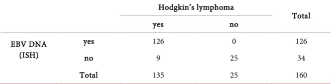
Dinand et al. [17] conducted a case control study to investigate the prevalence and significance of Epstein-Barr virus in Hodgkin’s and Reed-Sternberg cells in children. EBV detection was performed by immunohistochemistry (IHC) and in situ hybridization (ISH). Dinand et al. [17] detected EBV by ISH in 126/135 (93.3%) out of 135 cases, and in none 0/25 (0%) of the control lymph node ex-amined. The data as obtained 2007 by Dinand et al. are presented by the 2 by 2-table (Table 1).
DOI: 10.4236/jbm.2018.61008 77 Journal of Biosciences and Medicines
Table 1. Epstein-Barr virus (EBV) and Hodgkin’s lymphoma according to Dinand et al. (2007).
Hodgkin’s lymphoma
Total
yes no
EBV DNA (ISH)
yes 126 0 126
no 9 25 34
Total 135 25 160
ISH (FISH), RNA in situ hybridization (RNA ISH), Polymerase chain reaction (PCR), Nested PCR, Quantitative polymerase chain reaction (QPCR) have fueled us to change our understanding of the pathogenesis of cancer development. Immunohistochemistry (IHC), introduced by Coons [19] in 1941, is useful in distinguishing between benign and malignant cell populations. Still, a cross-reactivity with cellular proteins is possible which has impact on the specif-ity of this method. In situ hybridization (ISH) is a fundamental technique, de-scribed in the year 1969 by Joseph G. Gall [20] is used commonly for research purposes especially to distinguish virus in tumor cells from virus in non-tumor cells. Despite of numerous advantages, the use of the ISH technique is associated with certain and severe limitations. The skill of the personnel involved in per-forming and interpreting ISH has influence on the reproducibility and accuracy of this procedure. In situ hybridization (ISH) even if regarded as superior to PCR depend on the target used which has impact on the sensitivity and specific-ity of this methods. Even the In situ hybridization (ISH) can produce false posi-tive or false negaposi-tive results.
2.2. Study of Veronique Dinad
et al.
(2015)
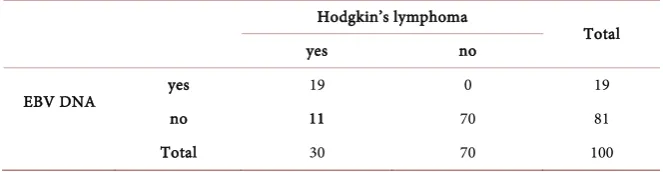
Veronique Dinand et al. [21] conducted a study to measure circulating EBV DNA in 30 children with Hodgkin lymphoma (HL) and in 70 controls, with prospective follow-up of the Hodgkin lymphoma cohort (2007-2012). Over the same time period, a cohort study monitored the HL cohort’s response to therapy, EBV load and long-term remission status. Pre-treatment quantitative EBV-DNA PCR was positive in 19 out of 30 children with Hodgkin lymphoma cases while all 70 controls were tested EBV quantitative PCR negative. The highest EBV load was 430,000 copies/mL. Out of 19 quantitative EBV-DNA PCR was positive children, one died of advanced disease before starting chemotherapy. The data as obtained 2015 by Dinand et al. are presented by the 2 by 2-table (Table 2).
2.3. Statistical Analysis
All statistical analyses were performed with Microsoft Excel version 14.0.7166.5000 (32-Bit) software (Microsoft GmbH, Munich, Germany).
2.3.1. Bernoulli Trials
DOI: 10.4236/jbm.2018.61008 78 Journal of Biosciences and Medicines
Table 2. Epstein-Barr virus (EBV) and Hodgkin’s lymphoma according to Dinand et al. (2015).
Hodgkin’s lymphoma
Total
yes no
EBV DNA yes 19 0 19
no 11 70 81
Total 30 70 100
Poisson distribution et cetera the binomial distribution is of special interest. Sometimes, the binomial distribution is called the Bernoulli distribution in hon-or of the Swiss mathematician Jakob Bernoulli (1654 - 1705), who derived the same. Bernoulli trials are an essential part of the Bernoulli distribution. Thus far, let us assume two fair coins named as 0Wt and as RUt. In our model, heads of
such a coin are considered as success T (i.e. true) and labeled as +1 while tails may be considered as failure F (i.e. false) and are labeled as +0. Such a coin is called a Bernoulli-Boole coin. The probability of success of RUt at one single
Bernoulli trial t is denoted as
(
R t 1)
(
R t)
p U = + ≡p U (1)
The probability of failure of RUt at one single Bernoulli trial t is denoted as
(
R t 0)
(
R t)
1(
R t)
p U = + ≡p U ≡ −p U (2)
Furthermore, no matter how many times an experiment is repeated, let the probability of a head or the tail remain the same. The trials are independent which implies that no matter how many times an experiment is repeated, the probability of a single event at a single trial remain the same. Repeated indepen-dent trials which are determined by the characteristic that there are always only two possible outcomes, either +1 or +0 and that the probability of an event (outcome) remain the same at each single trial for all trials are called Bernoulli trials. The definition of Bernoulli trials provides a theoretical model which is of further use. However, in many practical applications, we may by confronted by circumstances which may be considered as approximately satisfying Bernoulli trials. Thus far, let us perform an experiment of tossing two fair coins simulta-neously. Suppose two fair coins are tossed twice. Then there are 22 = 4 possible
outcomes (the sample space), which may be shown as
[
] [
]
(
)
(
[
] [
]
)
[
]
(
)
(
[
]
)
0 0
0 0
1 , 1 , 1 , 0 , 0, 1 , 0, 0
R t t R t t
R t t R t t
U W U W
U W U W
= + = + = + = +
= + = + = + = +
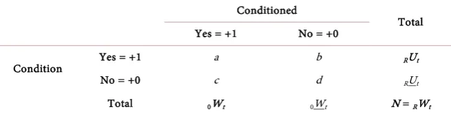
This may also be shown as a 2-dimensional sample space in the form of a con-tingency table (Table 3).
In the following, the contingency table is defined more precisely (Table 4). In general it is
(
a c+ =)
0Wt,(
a b+)
=RUt,(
c+d)
=0Wt,(
b+d)
= RUtand a+ + + =b c d N= RWt. Equally, it is 0Wt+0Wt = RUt +RUt = RWt =N.
DOI: 10.4236/jbm.2018.61008 79 Journal of Biosciences and Medicines
Table 3. The sample space of a contingency table.
Conditioned
Total
Yes = +1 No = +0
Condition Yes =+1 ([RUt = +1], [0Wt = +1]) ([RUt = +1], [0Wt = +0]) RUt No = +0 ([RUt = +0], [0Wt = +1]) ([RUt = +0], [0Wt = +0]) RUt
Total 0Wt 0Wt RWt
Table 4. The sample space of a contingency table.
Conditioned
Total Yes = +1 No = +0
Condition Yes = +1 a b RUt
No = +0 c d RUt
Total 0Wt 0Wt N = RWt
and an n dimensional sample space with 2n sample points is generated. In
gener-al, when given n Bernoulli trials with k successes, the probability to obtain ex-actly k successes in n Bernoulli trials is given by
( )
n(
R t 1)
k(
1(
R t 1)
)
n kp k p U p U
k
−
= × = + × − = +
(3)
The random variable k is sometimes called a binomial variable. The probabil-ity to obtain k events or more (at least k events) in n trials is calculated as
(
)
(
)
(
)
(
1)
(
1(
1)
)
k n n k
k
R t R t
k X
p k X p k X p k X
n
p U p U
k
= −
=
≥ = = + >
= × = + × − = +
∑
(4)The probability to obtain less than k events in n Bernoulli trials is calculated as
(
)
(
)
(
)
(
(
)
)
1
1 1 1 1
k n
n k k
R t R t
k X
p k X p k X
n
p U p U
k
= −
=
< = − ≥
= − × = + × − = +
∑
(5)2.3.2. Sufficient Condition (Conditio per Quam)
The formula of the conditio per quam [22]-[35] relationship was derived as
(
EBV DNA Hodgkin s lymphoma)
a c dp
N
+ +
→ ’ ≡ (6)
and used to proof the hypothesis: if presence of EBV infection (EBV DNA) then presence of Hodgkin’s lymphoma.
2.3.3. Necessary Condition (Conditio Sine Qua Non)
The formula of the conditio per quam [22]-[35] relationship was derived as
(
EBV DNA Hodgkin s lymphoma)
a b dp
N
+ +
DOI: 10.4236/jbm.2018.61008 80 Journal of Biosciences and Medicines and used to proof the hypothesis: without presence of EBV infection (EBV DNA) no presence of Hodgkin’s lymphoma.
2.3.4. Necessary and Sufficient Condition
The necessary and sufficient condition relationship was defined [22]-[35] as
(
EBV DNA Hodgkin s lymphoma)
a dp
N
+
←→ ’ ≡ (8)
Scholium.
Historically, the notion sufficient condition is known since thousands of years. Many authors testified original contributions of the notion material implication only for Diodorus Cronus. Still, Philo the Logician (~300 BC), a member of a group of early Hellenistic philosophers (the Dialectical school), is the main forerunner of the notion material implication and has made some groundbreak-ing contributions [36] to the basics of this relationship. As it turns out, it is very hard to think of the “conditio per quam” relationship without considering the historical background of this concept. Remarkable as it is, Philo’s concept of the material implications came very close to that of modern concept material impli-cation. In propositional logic, a conditional is generally symbolized as “p → q” or in spoken language “if p then q”. Both q and p are statements, with q the quent and p the antecedent. Many times, the logical relation between the conse-quent and the antecedent is called a material implication. In general, a condi-tional “if p then q” is false only if p is true and q is false otherwise, in the three other possible combinations, the conditional is always true. In other words, to say that p is a sufficient condition for q is to say that the presence of p guarantees the presence of q. In particular, it is impossible to have p without q. If p is present, then q must be present too. To show that p is not sufficient for q, we come up with cases where p is present but q is not. It is well-known that the no-tion of a necessary condino-tion can be used in defining what a sufficient condino-tion is (and vice versa). In general, p is a necessary condition for q if it is impossible to have q without p. In fact, the absence of p guarantees the absence of q. Exam-ple (Condition: Our earth), without oxygen no fire. Table 5 may demonstrate this relationship.
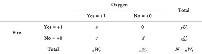
In contrast to such a point of view, the opposite point of view is correct too. Thus far, there is a straightforward way to give a precise and comprehensive ac-count of the meaning of the term necessary or sufficient condition itself. In other words, if fire is present then oxygen is present too. Table 6 may demonstrate this relationship.
Table 5. Without oxygen no fire (on our planet earth).
Fire
Total
Yes = +1 No = +0
Oxygen Yes = +1 a b RUt
No = +0 0 d RUt
DOI: 10.4236/jbm.2018.61008 81 Journal of Biosciences and Medicines
Table 6. If fire is present then oxygen is present too (on our planet earth).
Oxygen
Total
Yes = +1 No = +0
Fire Yes = +1 a 0 RUt
No = +0 c d RUt
Total 0Wt 0Wt N = RWt
Especially, necessary and sufficient conditions are converses of each other. Still, the fire is not the cause of oxygen and vice versa. Oxygen is note the cause of fire. In this example before, oxygen is a necessary condition, a conditio sine qua non, of fire. A necessary condition is sometimes also called “an essential condition” or a conditio sine qua non. In propositional logic, a necessary condi-tion, a condition sine qua non, is generally symbolized as “p ← q” or in spoken language “without p no q”. Both q and p are statements, with p the antecedent and q the consequent. To show that p is not a necessary condition for q, it is ne-cessary to find an event or circumstances where q is present (i.e. an illness) but p (i.e. a risk factor) is not. On any view, (classical) logic has as one of its goals to characterize the most basic, the most simple and the most general laws of objec-tive reality. Especially, in classical logic, the notions of necessary conditions, of sufficient conditions of necessary and sufficient conditions et cetera are defined very precisely for a single event, for a single Bernoulli trial t. In point of fact, no matter how many times an experiment is repeated, the relationship of the condi-tio sine qua or of the condicondi-tio per quam which is defined for every single event will remain the same. Under conditions of independent trials this implies that no matter how many times an experiment is repeated, the probability of the condi-tio sine qua or of the condicondi-tio per quam of a single event at a single trial t remain the same which transfers the relationship of the conditio sine qua or of the con-ditio per quam et cetera into the sphere of (Bio-) statistics. Consequently, (Bio) statistics generalizes the notions of a sufficient or of a necessary condition from one single Bernoulli trial to N Bernoulli trials. However, in many practical ap-plications, we may by confronted by circumstances which may be considered as approximately satisfying the notions of a sufficient or of a necessary condition. Thus far, under these circumstances, we will need to perform some tests to in-vestigate, can we rely on our investigation.
2.3.5. The Central Limit Theorem
DOI: 10.4236/jbm.2018.61008 82 Journal of Biosciences and Medicines such results? The concept of confidence intervals, closely related to statistical significance testing, was formulated to provide an answer to this problem.
Confidence intervals, introduced to statistics by Jerzy Neyman in a paper pub-lished in 1937 [37], specifies a range within a parameter, i.e. the population proportion π, with a certain probability, contain the desired parameter value. Most commonly, the 95% confidence interval is used. Interpreting a confidence interval involves a couple of important but subtle issues. In general, a 95% con-fidence interval for the value of a random number means that there is a 95% probability that the “true” value of the value of a random number is within the interval. Confidence intervals for proportions or a population mean of random variables which are not normally distributed in the population can be con-structed while relying on the central limit theorem as long as the sample sizes and counts are big enough (i.e. a sample size of n = 30 and more). A formula, justified by the central limit theorem, is known as
(
)
2 Alpha 2
1
1
Crit Calc Calc Calc
p p z p p
N
= ± × × × −
(9)
where pCalc is the sample proportion of successes in a Bernoulli trial process with
N trials yielding X successes and N-X failures and z is i.e. the 1 − (Alpha/2) quantile of a standard normal distribution corresponding to the significance lev-el alpha. For example, for a 95% confidence levlev-el alpha = 0.05 and z is z = 1.96. A very common technique for calculating binomial confidence intervals was pub-lished by Clopper-Pearson [38]. Agresti-Coull proposed another different me-thod [39] for calculating binomial confidence intervals. A faster and an alterna-tive way to determine the lower and upper “exact” confidence interval is justified by the F distribution [40].
2.3.6. The Rule of Three
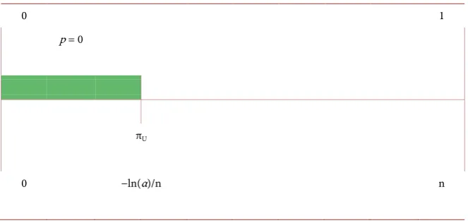
Furthermore, an approximate and conservative (one sided) confidence interval was developed by Louis [41], Hanley et al. [42] and Jovanovic [43] known as the rule of three. Briefly sketched, the rule of three can be derived from the binomial model. Let πU denote the upper limit of the one-sided 100 × (1 − α)% confidence
interval for the unknown proportion when in N independent trials no events occur [43]. Then πU is the value such that
( )
ln 3
U
n n
α
π =− ≈
(10) assuming that α = 0.05. In other words, an one-sided approximate upper 95% confidence bound for the true binomial population proportion π, the rate of oc-currences in the population, based on a sample of size n where no successes are observed (p = 0) is 3/n [43] or given approximately by [0 < π < (3/n)]. The rule of three is a useful tool especially in the analysis of medical studies. Table 7 will illustrate this relationship.
DOI: 10.4236/jbm.2018.61008 83 Journal of Biosciences and Medicines n subjects (i.e. p = 0) the interval from 0 to (−ln(α)/n) is called a 100 × (1 − α)% confidence interval for the binomial parameter for the rate of occurrences in the population.
Another special case of the binomial distribution is based on a sample of size n where only successes are observed (p = 1). Accordingly, the lower limit of a one-sided 100 × (1 − α)% confidence interval for a binomial probability πL, the
rate of occurrences in the population, based on a sample of size n where only successes are observed is given approximately by [(1− (−ln(α)/n)) < π < +1] or (assuming α = 0.05)
( )
ln 3
1 1
L
n n
α
π = −− ≈ −
(11) Table 8 may illustrate this relationship.
[image:9.595.209.541.369.527.2]To construct a two-sided 100 × (1 − (α))% interval according to the rule of three, it is necessary to take a one-sided 100 × (1 − (α/2))% confidence interval. In this study, we will use the rule of three [44] too, to calculate the confidence interval for the value of a random number.
Table 7. The one-sided approximate upper 100 × (1 − α)% confidence bound where no successes (p = 0) are observed.
0 1
p = 0
πU
0 −ln(α)/n n
Table 8. The one-sided approximate upper 100 × (1 − α)% confidence bound where only successes are observed.
0 +1
p = 1
πL
DOI: 10.4236/jbm.2018.61008 84 Journal of Biosciences and Medicines 2.3.7. Fisher’s Exact Test
A test statistics of independent and more or less normally distributed data which follow a chi-squared distribution is valid as with many statistical tests due to the central limit theorem. Especially, with large samples, a chi-squared distribution can be used. A sample is considered as large when the sample size n is n = 30 or more. With a small sample (n < 30), the central limit theorem does not apply and erroneous results could potentially be obtained from the few observations if the same is applied. Thus far, when the number of observations obtained from a population is too small, a more appropriate test for of analysis of categorical data i.e. contingency tables is R. A. Fisher’s exact test [45]. Fisher’s exact test is valid for all sample sizes and calculates the significance of the p-value (i.e. the devia-tion from a null hypothesis) exactly even if in practice it is employed when sam-ple size is small. Fisher’s exact test is called exact because the same uses the exact hypergeometric distribution to compute the p-value rather than the approximate chi-square distribution. Still, computations involved in Fisher’s exact test can be time consuming to calculate by hand.
2.3.8. Hypergeometric Distribution
The hypergeometric distribution, illustrated in a table (Table 9), is a discrete probability distribution which describes the probability of a events/successes in a sample with the size 0Wt, without replacement, from a finite population of the
size N which contains exactly RUt objects with a certain feature while each event
is either a success or a failure. The formula for the hypergeometric distribution, a discrete probability distribution, is
( )
00
R t
R t
t
t
N U
U
W a
a p a
N
W −
×
−
=
(12)
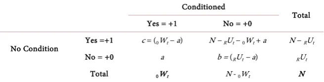
The hypergeometric distribution has a wide range of applications. The Hypergeometric distribution can be approximated by a Binomial distribution. The elements of the population being sampled are classified into one of two mutually exclusive categories: either conditio sine qua non or no conditio sine qua non relationship. We are sampling without replacement from a finite popu-lation. How probable is it to draw specific c events/successes out of 0Wt total
draws from an aforementioned population of the size N? The hypergeometric distribution, as shown in a table (Table 10) is of use to calculate how probable is it to obtain c = (0Wt − a) events out of N events.
Table 9. The hypergeometric distribution.
Conditioned
Total
Yes = +1 No = +0
Condition Yes = +1 a b =(RUt – a) RUt
No = +0 c = (0Wt − a) N − RUt − 0Wt + a N − RUt
DOI: 10.4236/jbm.2018.61008 85 Journal of Biosciences and Medicines
Table 10. The hypergeometric distribution and conditio sine qua non.
Conditioned
Total
Yes = +1 No = +0
No Condition Yes =+1 c = (0Wt − a) N − RUt − 0Wt + a N − RUt
No = +0 a b = (RUt − a) RUt
Total 0Wt N - 0Wt N
2.3.9. Statistical Hypothesis Testing
A statistical hypothesis test is a method to extract some inferences from data. A hypothesis is compared as an alternative hypothesis. Under which conditions does the outcomes of a study lead to a rejection of the null hypothesis for a pre-specified level of significance. According to the rules of a proof by contra-diction, a null hypothesis (H0) is a statement which one seeks to disproof. The
related specific alternative hypothesis (HA) is opposed to the null hypothesis
such that if null hypothesis (H0) is true, the alternative hypothesis (HA) is false
and vice versa. If the alternative hypothesis (HA) is true then the null hypothesis (H0) is false. In principle, a null hypothesis that is true can be rejected (type I
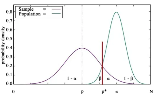
er-ror) which lead us to falsely infer the existence of something which is not given. The significance level, also denoted as α (alpha) is the probability of rejecting a null hypothesis when the same is true. A type II error is given, if we falsely infer the absence of something which in reality is given. A null hypothesis can be false but a statistical test may fail to reject such a false null hypothesis. The probability of accepting a null hypothesis when the same is false (type II error), is denoted by the Greek letter β (beta) and related to the power of a test (which equals 1 − β). The power of a test indicates the probability by which the test correctly re-jects the null hypothesis (H0) when a specific alternative hypothesis (HA) is true.
Most investigator assess the power of a tests using 1 − β = 0.80 as a standard for adequacy. A tabularized relation between truth/falseness of the null hypothesis and outcomes of the test are shown precisely within a table (Table 11).
In general, it is 1 − α + α = 1 or (1 − α − β) + α = 1− β. Figure 1 may illustrate these relationships.
2.3.10. The Mathematical Formula of the Causal Relationship k The mathematical formula of the causal relationship k [22]-[35] defined as
(
)
(
(
) (
)
)
(
) (
)
0 0
2
0 0
, R t t
R t t
R t R t t
N a U W
k U W
U U W W
× − ×
≡
DOI: 10.4236/jbm.2018.61008 86 Journal of Biosciences and Medicines
Figure 1. The relationship between error types.
Table 11. Table of error types.
Null Hypothesis (H0) is
Total
True False
Null Hypothesis (H0)
Accepted 1 − α β 1 −α + β
Rejected α 1 − β 1 +α − β
Total 1 1 2
[image:12.595.210.540.274.351.2]DOI: 10.4236/jbm.2018.61008 87 Journal of Biosciences and Medicines causal relationship (Bradford Hill criteria). In point of fact, Bredford’s “fourth characteristic is the temporal relationship of the association” [49] and in last consequence the “post hoc ergo propter hoc” logical fallacy. Causation cannot be derived from the “post hoc ergo propter hoc” [35] logical fallacy. Consequently, the Mathematical Formula of the causal relationship k can neither be reduced to the Bradford Hill criteria nor is the same just a mathematization of Bradford Hill criteria.
2.3.11. The Chi Square Distribution
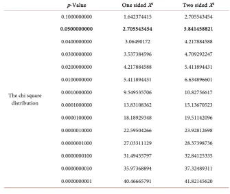
The chi-squared distribution [46] is a widely known distribution and used in hypothesis testing, in inferential statistics or in construction of confidence in-tervals. The critical values of the chi square distribution are visualized by Table 12.
2.3.12. The X2 Goodness of Fit Test
A chi-square goodness of fit test can be applied to determine whether sample data are consistent with a hypothesized distribution. The chi-square goodness of fit test is appropriate when some conditions are met. A view of these conditions are simple random sampling, categorical variables and an expected value of the number of sample observations which is at least 5. The null hypothesis (H0) and
its own alternative hypothesis (HA) are stated in such a way that they are
mu-tually exclusive. In point of fact, if the null hypothesis (H0) is true, the other,
al-ternative hypothesis (HA), must be false; and vice versa. For a chi-square
[image:13.595.204.540.449.731.2]good-ness of fit test, the hypotheses can take the following form.
Table 12. The critical values of the chi square distribution (degrees of freedom: 1).
p-Value One sided X2 Two sided X2
The chi square distribution
0.1000000000 1.642374415 2.705543454 0.0500000000 2.705543454 3.841458821
DOI: 10.4236/jbm.2018.61008 88 Journal of Biosciences and Medicines H0: The sample distribution agrees with the hypothetical (theoretical)
distri-bution.
HA: The sample distribution does not agree with the hypothetical (theoretical)
distribution.
The X2 Goodness-of-Fit Test can be shown schematically as
(
)
22
1
Observed Expected
Expected
t N
t t
t t
χ =+
=+
−
≡
∑
(14)The degrees of freedom are calculated as N − 1. If there is no discrepancy be-tween an observed and a theoretical distribution, then X2 = 0. As the discrepancy
between an observed and a theoretical distribution becomes larger, the X2
be-comes larger. This X2 values are evaluated by the known X2 distribution.
The original X2 values are calculated from an original theoretical distribution,
which is continuous, whereas the approximation by the X2 Goodness of fit test
we are using is discrete. Thus far, there is a tendency to underestimate the prob-ability, which means that the number of rejections of the null hypothesis can in-crease too much and must be corrected downward. Such an adjustment (Yate’s correction for continuity) is used only when there is one degree of freedom. When there is more than one degree of freedom, the same adjustment is not used. Applying this to the formula above, we find the X2 Goodness-of-Fit Test
with continuity correction shown schematically as
2
2 1
1 Observed Expected
2 Expected
t t
t N
t t
χ =+
=+
− −
≡
∑
(15)When the term (|Observedt − Expectedt|) is less than 1/2, the continuity
cor-rection should be omitted.
1) The X² Goodness of Fit Test of a Sufficient Condition
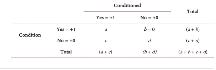
The theoretical (hypothetical) distribution of a sufficient condition is shown schematically by the 2 × 2 table (Table 13).
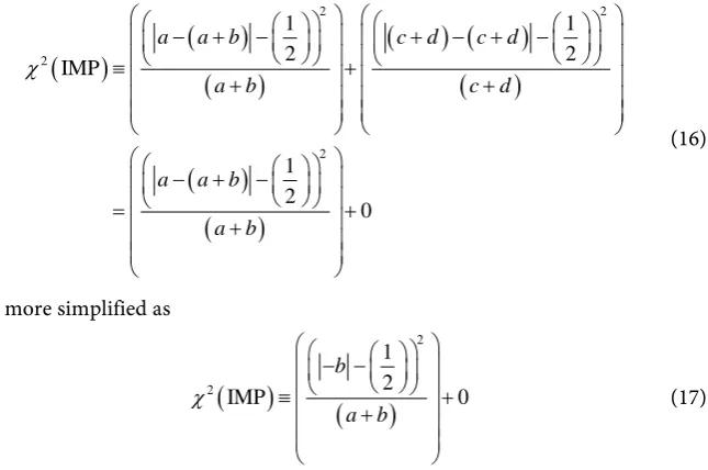
The theoretical distribution of a sufficient condition (conditio pre quam) is determined by the fact that b = 0. The X2 Goodness-of-Fit Test with continuity
[image:14.595.191.541.627.741.2]correction of a sufficient condition (conditio per quam) is calculated as
Table 13. The theoretical distribution of a sufficient condition (conditio pre quam).
Conditioned
Total Yes = +1 No = +0
Condition Yes = +1 a b = 0 (a + b)
No = +0 c d (c + d)
DOI: 10.4236/jbm.2018.61008 89 Journal of Biosciences and Medicines
(
)
(
(
)
)
(
) (
(
)
)
(
)
(
)
2 2 2 2 1 1 2 2 IMP 1 2 0a a b c d c d
a b c d
a a b
a b χ − + − + − + − ≡ + + + − + − = + + (16)
or more simplified as
(
)
(
)
2 2 1 2 IMP 0 b a b χ − − ≡ + + (17)Under these circumstances, the degree of freedom is d.f. = N− = − =1 2 1 1.
2) The X2 goodness of fit test of a necessary condition
The theoretical (hypothetical) distribution of a necessary condition is shown schematically by the 2 × 2 table (Table 14).
The theoretical distribution of a necessary condition (conditio sine qua non) is determined by the fact that c = 0. The X2 Goodness-of-Fit Test with continuity
correction of a necessary condition (conditio sine qua non) is calculated as
(
)
(
) (
(
)
)
( ) (
(
)
)
(
)
(
)
2 2 2 2 1 1 2 2 SINE 1 2 0a b a b d c d
a b c d
d c d
c d χ + − + − − + − ≡ + + + − + − = + + (18)
or more simplified as
[image:15.595.216.539.72.286.2](
)
(
)
2 2 1 2 SINE 0 c c d χ − − ≡ + + (19)Table 14. The theoretical distribution of a necessary condition (conditio sine qua non).
Conditioned
Total Yes = +1 No = +0
Condition Yes = +1 a b (a + b)
No = +0 c = 0 d (c + d)
DOI: 10.4236/jbm.2018.61008 90 Journal of Biosciences and Medicines Under these circumstances, the degree of freedom is d.f. = N− = − =1 2 1 1.
3) The X2 goodness of fit test of a necessary and sufficient condition
The theoretical (hypothetical) distribution of a necessary and sufficient condi-tion is shown schematically by the 2 × 2 table (Table 15).
The theoretical distribution of a necessary and sufficient condition is deter-mined by the fact that b = 0 and that c = 0. The X2 Goodness-of-Fit Test with
continuity correction of a necessary and sufficient condition is calculated as
(
)
( ) (
)
(
)
( ) (
)
(
)
2
2 2
Necessary AND Sufficient
1 1
2 2
a a b d c d
a b c d
χ
− + − − + −
≡ +
+ +
(20)
or more simplified as
(
)
(
)
(
)
2 2
2
1 1
2 2
Necessary AND Sufficient
b c
a b c d
χ
− − − −
≡ +
+ +
(21)
Under these circumstances, the degree of freedom is d.f. = N− = − =1 2 1 1.
3. Results
3.1. Epstein-Bar Virus Is a
Conditio sine qua
Non of Hodgkin’s
Lymphoma
Claims.
Null hypothesis:
An infection of human lymph nodes by Epstein-Bar virus is a conditio sine qua non of Hodgkin’s lymphoma.
Alternative hypothesis:
An infection of human lymph nodes by Epstein-Bar virus is not a conditio sine qua non of Hodgkin’s lymphoma.
Significance level (Alpha) below which the null hypothesis will be rejected: 0.05.
Proof.
[image:16.595.207.540.640.737.2]The data of an infection by Epstein-Bar virus and Hodgkin’s lymphoma are viewed in the 2 × 2 table (Table 1). The X2 Goodness-of-Fit Test with continuity
Table 15. The theoretical distribution of a necessary and sufficient condition.
Conditioned
Total Yes = +1 No = +0
Condition Yes = +1 a b = 0 (a + b)
No = +0 c = 0 d (c + d)
DOI: 10.4236/jbm.2018.61008 91 Journal of Biosciences and Medicines correction of a necessary condition (conditio sine qua non) known to be defined as p (Epstein-Bar virus DNA ← Hodgkin’s lymphoma) is calculated as
(
)
(
)
(
)
2 2
2
1 1
9
2 2
SINE 0 2.125
9 25
c
c d
χ
− − − −
≡ + = =
+ +
Under these circumstances, the degree of freedom is d.f. = N− = − =1 2 1 1.
The critical X2 (significance level alpha = 0.05) is known to be 3.841458821
(Table 12). The calculated X2 value = 2.125 and less than the critical X2 =
3.841458821. Hence, our calculated X2 value = 2.125 is not significant and we
accept our null hypothesis. Due to this evidence, we do not reject the null hypo-thesis in favor of the alternative hypotheses. In other words, the sample distribu-tion agrees with the hypothetical (theoretical) distribudistribu-tion. Our hypothetical distribution was the distribution of the necessary condition. Thus far, the data as published by Dinand et al. [17] do support our null hypothesis that an infection of human lymph nodes by Epstein-Bar virus is a conditio sine qua non of Hodg-kin’s lymphoma. In other words, without an infection of human lymph nodes by Epstein-Bar virus no Hodgkin’s lymphoma.
Q.e.d.
3.2. Epstein-Bar Virus Is a
Conditio per quam
of Hodgkin’s
Lymphoma
Claims.
Null hypothesis:
An infection of human lymph nodes by Epstein-Bar virus is a conditio per quam of Hodgkin’s lymphoma.
(p0 > pCrit).
Alternative hypothesis:
An infection of human lymph nodes by Epstein-Bar virus is not a conditio per quam of Hodgkin’s lymphoma.
(p0 < pCrit).
Significance level (Alpha) below which the null hypothesis will be rejected: 0.05.
Proof.
The data of an infection by Epstein-Bar virus and Hodgkin’s lymphoma are viewed in the 2 × 2 table (Table 1). The proportion of successes in the sample of a conditio per quam relationship p (Epstein-Bar virus DNA → Hodgkin’s lym-phoma) is calculated [22]-[35] as
(
) (
126 9 25)
160 EBV DNA Hodgkin s lymphoma 1160 160
p → ’ = + + = =
The critical value pCrit (significance level alpha = 0.05) is calculated [39]-[44]
DOI: 10.4236/jbm.2018.61008 92 Journal of Biosciences and Medicines
3
1 0.981276673 160
Crit
p = − =
The critical value is pCrit = 0.981276673 and is less than the proportion of
suc-cesses calculated as p (Epstein-Bar virus DNA → Hodgkin’s lymphoma) = 1. Due to this evidence, we do not reject the null hypothesis in favor of the alternative hypotheses. The data as published by Dinand et al. [17] do support our Null hy-pothesis that an infection of human lymph nodes by Epstein-Bar virus is a con-ditio per quam of Hodgkin’s lymphoma. In other words, if an infection of hu-man lymph nodes by Epstein-Bar virus is present then Hodgkin’s lymphoma is present too.
Q.e.d.
3.3. Epstein-Bar Virus Is the Cause of Hodgkin’s Lymphoma
Claims.
Null hypothesis: (no causal relationship)
There is no causal relationship between an infection of human lymph nodes by Epstein-Bar virus and Hodgkin’s lymphoma.
Alternative hypothesis: (causal relationship)
There is a causal relationship between an infection of human lymph nodes by Epstein-Bar virus and Hodgkin’s lymphoma.
(k <> 0). Conditions. Alpha level = 5%.
The two tailed critical Chi square value (degrees of freedom = 1) for alpha lev-el 5% is 3.841458821.
Proof.
The data for this hypothesis test are illustrated in the 2 × 2 table (Table 1). The causal relationship k (EBV DNA, Hodgkin’s lymphoma) is calculated [22]-[35] as
(
)
(
) (
)
(
)
(
) (
)
2
EBV DNA, Hodgkin s lymphoma
160 126 126 135
0.82841687 126 34 135 25
k
× − ×
= = +
× × ×
’
The value of the test statistic k = +0.82841687 is equivalent to a calculated [22]-[35] chi-square value of
(
) (
)
(
)
(
) (
)
(
) (
)
(
)
(
) (
)
2 Calculated
2 2
2 Calculated
2 Calculated
160 126 126 135 160 126 126 135 160
126 34 135 25 126 34 135 25 160 0.82841687 0.82841687
109.8039216
χ
χ χ
× − × × − ×
= × ×
× × × × × ×
= × ×
=
The chi-square statistic, uncorrected for continuity, is calculated as X2 =
109.8039216 and thus far equivalent to a P value of
DOI: 10.4236/jbm.2018.61008 93 Journal of Biosciences and Medicines the null hypothesis and accept the alternative hypotheses. There is a highly sig-nificant causal relationship between an infection of human lymph nodes by Eps-tein-Bar virus and Hodgkin’s lymphoma (k = +0.82841687, p Value =
0.000000000000000000000000108179). The result is significant at p < 0.001. Q.e.d.
3.4. Epstein-Bar Virus Is a
Conditio sine qua
Non of Hodgkin’s
Lymphoma
Claims.
Null hypothesis:
An infection of human lymph nodes by Epstein-Bar virus is a conditio sine qua non of Hodgkin’s lymphoma.
Alternative hypothesis:
An infection of human lymph nodes by Epstein-Bar virus is not a conditio sine qua non of Hodgkin’s lymphoma.
Significance level (Alpha) below which the null hypothesis will be rejected: 0.05.
Proof.
The data of an infection by Epstein-Bar virus and Hodgkin’s lymphoma are viewed in the 2 × 2 table (Table 2). The X2 Goodness-of-Fit Test with continuity
correction of a necessary condition (conditio sine qua non) known to be defined as p (Epstein-Bar virus DNA ← Hodgkin’s lymphoma) [22]-[35] is calculated as
(
)
(
)
(
)
2 2
2
1 1
11
2 2
SINE 0 1.361111111 11 70
c
c d
χ
− − − −
≡ + = =
+ +
(22)
Under these circumstances, the degree of freedom is d.f. = N− = − =1 2 1 1.
The critical X2 (significance level alpha = 0.05) is known to be 3.841458821
(Table 12). The calculated X2 value is 1.361111111and is less than the critical
X2 = 3.841458821. Hence, our calculated X2 value is 1.361111111 and is not
sig-nificant and we accept the null hypothesis. Due to this evidence, we do not reject the null hypothesis in favor of the alternative hypotheses. In other words, the sample distribution agrees with the hypothetical (theoretical) distribution. Our hypothetical distribution was the distribution of the necessary condition. Thus far, the data as published by Dinand et al. [21] do support our null hypothesis that an infection of human lymph nodes by Epstein-Bar virus is a conditio sine qua non of Hodgkin’s lymphoma. In other words, without an infection of hu-man lymph nodes by Epstein-Bar virus no Hodgkin’s lymphoma.
Q.e.d.
3.5. An Infection of Human Lymph Nodes by Epstein-Bar Virus Is a
Conditio per quam
of Hodgkin’s Lymphoma
DOI: 10.4236/jbm.2018.61008 94 Journal of Biosciences and Medicines Null hypothesis:
An infection of human lymph nodes by Epstein-Bar virus is a conditio per quam of Hodgkin’s lymphoma.
(p0 > pCrit).
Alternative hypothesis:
An infection of human lymph nodes by Epstein-Bar virus is not a conditio per quam of Hodgkin’s lymphoma.
(p0 < pCrit).
Significance level (Alpha) below which the null hypothesis will be rejected: 0.05.
Proof.
The data of an infection by Epstein-Bar virus and Hodgkin’s lymphoma are viewed in the 2 × 2 table (Table 2). The proportion of successes in the sample of a conditio per quam relationship p(Epstein-Bar virus DNA → Hodgkin’s lym-phoma) is calculated [22]-[35] as
(
) (
19 11 70)
100 EBV DNA Hodgkin s lymphoma 1100 100
p → ’ = + + = =
The critical value pCrit (significance level alpha = 0.05) is calculated [39]-[44]
as
3 1 0.97
100
Crit
p = − =
The critical value is pCrit = 0.97 and is less than the proportion of successes
calculated as p(Epstein-Bar virus DNA → Hodgkin’s lymphoma) = 1. Due to this evidence, we do not reject the null hypothesis in favor of the alternative hypo-theses. The data as published by Dinand et al. [21] do support our Null hypothe-sis that an infection of human lymph nodes by Epstein-Bar virus is a conditio per quam of Hodgkin’s lymphoma. In other words, if an infection of human lymph nodes by Epstein-Bar virus then Hodgkin’s lymphoma.
Q.e.d.
3.6. Epstein-Bar Virus Is the Cause of Hodgkin’s Lymphoma
Claims.
Null hypothesis: (no causal relationship)
There is no causal relationship between an infection of human lymph nodes by Epstein-Bar virus and Hodgkin’s lymphoma.
Alternative hypothesis: (causal relationship)
There is a causal relationship between an infection of human lymph nodes by Epstein-Bar virus and Hodgkin’s lymphoma.
(k<>0). Conditions. Alpha level = 5%.
DOI: 10.4236/jbm.2018.61008 95 Journal of Biosciences and Medicines Proof.
The data for this hypothesis test are illustrated in the 2 × 2 table (Table 2). The causal relationship k (EBV DNA, Hodgkin’s lymphoma) is calculated [22]-[35] as
(
)
(
) (
)
(
)
(
) (
)
2
EBV DNA, Hodgkin s lymphoma
100 19 30 19
0.739814235 30 70 19 81
k
× − ×
= = +
× × ×
’
The value of the test statistic k = +0.739814235 is equivalent to a calculated [22]-[35] chi-square value of
(
) (
)
(
)
(
) (
)
(
) (
)
(
)
(
) (
)
2 Calculated
2 2
2 Calculated 2 Calculated
100 19 30 19 100 19 30 19 100
30 70 19 81 30 70 19 81
100 0.739814235 0.739814235
54.7325102881
χ
χ χ
× − × × − ×
= × ×
× × × × × ×
= × ×
=
The chi-square statistic, uncorrected for continuity, is calculated as X2 =
54.7325102881 and thus far equivalent to a P value of 0.000000000000138. The calculated chi-square statistic exceeds the critical chi-square value of 3.841458821 (Table 12). Consequently, we reject the null hypothesis and accept the alterna-tive hypotheses. There is a highly significant causal relationship between an in-fection of human lymph nodes by Epstein-Bar virus and Hodgkin’s lymphoma (k = +0.739814235, p Value = 0.000000000000138). The result is significant at p < 0.001.
Q.e.d.
4. Discussion
DOI: 10.4236/jbm.2018.61008 96 Journal of Biosciences and Medicines by secondary literature [50]. Despite of the view disadvantages of case-control studies discussed above, Dinand et al. [17] [21] detected EBV DNA by in situ hybridization (ISH), which cannot be ignored. The in situ hybridization, like any method, is not completely free of bias and is labeled with some severe limi-tations. Still, the in situ hybridization provides the opportunity to distinguish EBV DNA in tumor cells from EBV DNA in non-tumor cells. In general, it is known that a great proportion of HL tissues is able to harbor EBV within tumor cells. Emerging evidence suggests that EBV is causality related to Hodgkin’s lymphoma. According to the data as published by Dinand et al. [17], without an infection of human lymph nodes by Epstein-Bar virus no Hodgkin’s lymphoma. In the same context, there is a highly significant causal relationship between an infection of human lymph nodes by Epstein-Bar virus and Hodgkin’s lymphoma (k = +0.82841687, p-value = 0.000000000000000000000000108179). Thus far, Epstein-Bar virus is not only a cause, but the cause of Hodgkin’s lymphoma. The challenge is to unravel this complexity of the relationship between Epstein Bar virus and Hodgkin’s lymphoma by detailed consideration of the function of EBV genes in the appropriate (tumor) cellular context. The hope is justified that this approach has revealed the most fundamental aspects of HL pathogenesis and that the same has paved the way for a more targeted and individual therapies for HL patients. Even if EBV is the cause of HL, many times a specific therapy is not indicated for most patients with an EBV infection. In point of fact, some drugs, i. e. acyclovir, are able to inhibit EBV replication and to reduce viral shedding. Sometimes, corticosteroid therapy is considered for patients with severe com-plications of an EBV infection and is able to shorten the duration of some symptoms and fever associated with an EBV infection. In point of fact, vaccina-tion against EBV might be useful especially for people who are seronegative for EBV. In this context, preliminary studies in which EBV-seronegative children were vaccinated with vaccinia virus expressing gp350 where to some extent ef-fective [51] [52].
5. Conclusion
Epstein-Bar virus is the cause of Hodgkin’s lymphoma (k = +0.82841687, p Val-ue = 0.000000000000000000000000108179).
Acknowledgements
The public domain software GnuPlot was used to draw the figure.
References
[1] Epstein, M.A., Achong, B.G. and Barr, Y.M. (1964) Virus Particles in Cultured Lymphoblasts from Burkitt’s Lymphoma. Lancet, 283, 702-703.
https://doi.org/10.1016/S0140-6736(64)91524-7
DOI: 10.4236/jbm.2018.61008 97 Journal of Biosciences and Medicines
[3] Meij, P., Vervoort, M.B., Aarbiou, J., van Dissel, P., Brink, A., Bloemena, E., Meijer, C.J. and Middeldorp, J. (1999) Restricted Low-Level Human Antibody Responses against Epstein—Barr Virus (EBV)—Encoded Latent Membrane Protein 1 in a Subgroup of Patients with EBV-Associated Diseases. The Journal of Infectious Dis-eases, 179, 1108-1115. https://doi.org/10.1086/314704
[4] zur Hausen, H., Schulte-Holthausen, H., Klein, G., Henle, W., Henle, G., Clifford, P. and Santesson, L. (1970) EBV DNA in Biopsies of Burkitt Tumours and Anaplastic Carcinomas of the Nasopharynx. Nature, 228, 1056-1058.
https://doi.org/10.1038/2281056a0
[5] Golden, R.L. (1968) Infectious Mononucleosis with Epstein-Barr Virus Antibodies in Older Ages. JAMA: The Journal of the American Medical Association, 205, 595.
https://doi.org/10.1001/jama.1968.03140340065021
[6] Kapatai, G. and Murray, P. (2007) Contribution of the Epstein-Barr Virus to the Molecular Pathogenesis of Hodgkin Lymphoma. Journal of Clinical Pathology, 60, 1342-1349. https://doi.org/10.1136/jcp.2007.050146
[7] Hodgkin, T. (1832) On Some Morbid Experiences of the Absorbent Glands and Spleen. Medico-Chirurgical Transactions, 17, 69-97.
https://www.ncbi.nlm.nih.gov/pmc/articles/PMC2116706/
[8] Harris, N.L., Jaffe, E.S., Stein, H., Banks, P.M., Chan, J.K., Cleary, M.L., Delsol, G., De Wolf-Peeters, C., Falini, B., Gatter, K.C., et al. (1994) A Revised Euro-pean-American Classification of Lymphoid Neoplasms: A Proposal from the Inter-national Lymphoma Study Group. Blood, 84, 1361-1392.
https://www.ncbi.nlm.nih.gov/pubmed/8068936
[9] Sternberg, C. (1898) Über Eine Eigenartige Unter Dem Bilde Der Pseudoleukamie Verlaufende Tuberculose Des Lymphatischen Apparates. Zeitschrift für Heilkunde, 19, 21-90.
[10] Reed, D. (1902) On the Pathological Changes in Hodgkin’s Disease, with Special Reference to Its Relation to Tuberculosis. The Johns Hopkins Hospital Reports, 10, 133-196.
[11] Küppers, R., Rajewsky, K., Zhao, M., Simons, G., Laumann, R., Fischer, R. and Hansmann, M.L. (1994) Hodgkin Disease: Hodgkin and Reed-Sternberg Cells Picked from Histological Sections Show Clonal Immunoglobulin Gene Rearrange-ments and Appear to Be Derived from B Cells at Various Stages of Development. Proceedings of the National Academy of Sciences of the United States of America, 91, 10962-10966.https://doi.org/10.1073/pnas.91.23.10962
[12] Newell, G.R. and Rawlings, W. (1972) Evidence for Environmental Factors in the Etiology of Hodgkin’s Disease. Journal of Chronic Diseases, 25, 261-267.
https://doi.org/10.1016/0021-9681(72)90162-2
[13] Goldman, J.M. and Aisenberg, A.C. (1970) Incidence of Antibody to EB Virus, Herpes Simplex, and Cytomegalovirus in Hodgkin’s Disease. Cancer, 26, 327-331. https://doi.org/10.1002/1097-0142(197008)26:2<327::AID-CNCR2820260213>3.0.C O;2-8
[14] Levine, P.H. (1970) E.B. Virus and Lymphomas. Lancet, 296, 771.
https://doi.org/10.1016/S0140-6736(70)90243-6
[15] Levine, P.H., Ablashi, D.V., Berard, C.W., et al. (1971) Elevated Antibody Titers to Epstein-Barr Virus in Hodgkin’s Disease. Cancer, 27, 416-421.
DOI: 10.4236/jbm.2018.61008 98 Journal of Biosciences and Medicines
[16] Weiss, L.M., Strickler, J.G., Warnke, R.A., Purtilo, D.T. and Sklar, J. (1987) Eps-tein-Barr Viral DNA in Tissues of Hodgkin’s Disease. American Journal of Pathol-ogy, 129, 86-91.https://www.ncbi.nlm.nih.gov/pmc/articles/PMC1899692/ [17] Dinand, V., Dawar, R., Arya, L.S., Unni, R., Mohanty, B. and Singh, R. (2007)
Hodgkin’s Lymphoma in Indian Children: Prevalence and Significance of Eps-tein-Barr Virus Detection in Hodgkin’s and Reed-Sternberg Cells. European Journal of Cancer, 43, 161-168. https://doi.org/10.1016/j.ejca.2006.08.036
[18] Chae, Y.K., Arya, A., Chiec, L., Shah, H., Rosenberg, A., Patel, S., Raparia, K., Choi, J., Wainwright, D.A., Villaflor, V., Cristofanilli, M. and Giles, F. (2017) Challenges and Future of Biomarker Tests in the Era of Precision Oncology: Can We Rely on Immunohistochemistry (IHC) or Fluorescence In Situ Hybridization (FISH) to Se-lect the Optimal Patients for Matched Therapy? Oncotarget, 8, 100863-100898.
https://doi.org/10.18632/oncotarget.19809
[19] Coons, A.H., Creech, H.J. and Jones, R.N. (1941) Immunological Properties of an Antibody Containing a Fluorescent Group. Experimental Biology and Medicine, 47, 200-202. https://doi.org/10.3181/00379727-47-13084p
[20] Gall, J.G. and Pardue, M.L. (1969) Formation and Detection of RNA-DNA Hybrid Molecules in Cytological Preparations. Proceedings of the National Academy of Sciences of the United States of America, 63, 378-383.
https://doi.org/10.1073/pnas.63.2.378
[21] Dinand, V., Sachdeva, A., Datta, S., Bhalla, S., Kalra, M., Wattal, C. and Radha-krishnan, N. (2015) Plasma Epstein Barr Virus (EBV) DNA as a biomarker for EBV-Associated Hodgkin Lymphoma. Indian Pediatrics, 52, 681-685.
https://doi.org/10.1007/s13312-015-0696-9
[22] Barukčić, I. (1989) Die Kausalität. Wissenschaftsverlag, Hamburg, 218. [23] Barukčić, I. (1997) Die Kausalität. Scientia, Wilhelmshaven, 374.
[24] Barukčić, I. (2005) Causality. New Statistical Methods. Books on Demand, Nor-derstedt, 488.
[25] Barukčić, I. (2006) Causality. New Statistical Methods. Second English Edition, Books on Demand, Norderstedt, 488.
[26] Barukčić, I. (2006) New Method for Calculating Causal Relationships. Proceeding of XXIIIrd International Biometric Conference, McGill University, Montréal, 16-21
Ju-ly 2006, 49.
[27] Barukčić, I. (2011) Causality I. A Theory of Energy, Time and Space. Lulu, Morris-ville,NC, 648.
[28] Barukčić, I. (2011) Causality II. A Theory of Energy, Time and Space. Lulu, Morris-ville, NC, 376.
[29] Barukčić, I. (2012) The Deterministic Relationship between Cause and Effect. In-ternational Biometric Conference, Kobe, Japan, 26-31 August 2012.
https://www.biometricsociety.org/conference-abstracts/2012/programme/p1-5/P-1/ 249-P-1-30.pdf
[30] Barukčić, I. (2016) The Mathematical Formula of the Causal Relationship k. Inter-national Journal of Applied Physics and Mathematics, 6, 45-65.
https://doi.org/10.17706/ijapm.2016.6.2.45-65
[31] Barukčić, K. and Barukčić, I. (2016) Epstein Barr Virus—The Cause of Multiple Sclerosis. Journal of Applied Mathematics and Physics, 4, 1042-1053.
https://doi.org/10.4236/jamp.2016.46109
DOI: 10.4236/jbm.2018.61008 99 Journal of Biosciences and Medicines
[33] Barukčić, I. (2017) Helicobacter pylori—The Cause of Human Gastric Cancer. Journal of Biosciences and Medicines,5, 1-19.
https://doi.org/10.4236/jbm.2017.52001
[34] Barukčić, I. (2017) Anti Bohr—Quantum Theory and Causality. International Journal of Applied Physics and Mathematics, 7, 93-111.
https://doi.org/10.17706/ijapm.2017.7.2.93-111
[35] Barukčić, I. (2017) Theoriae Causalitatis Principia Mathematica. Books on Demand, Norderstedt, 244.
https://www.bod.de/buchshop/theoriae-causalitatis-principia-mathematica-ilija-bar ukcic-9783744815932
[36] Astorga, M.L. (2015) Diodorus Cronus and Philo of Megara: Two Accounts of the Conditional. Rupkatha Journal on Interdisciplinary Studies in Humanities, 7, 9-16. [37] Neyman, J. (1937) Outline of a Theory of Statistical Estimation Based on the
Clas-sical Theory of Probability. Philosophical Transactions of the Royal Society A, 236, 333-380. https://doi.org/10.1098/rsta.1937.0005
[38] Clopper, C. and Pearson, E.S. (1934) The Use of Confidence or Fiducial Limits Illu-strated in the Case of the Binomial. Biometrika, 26, 404-413.
https://doi.org/10.1093/biomet/26.4.404
[39] Agresti, A. and Coull, B.A. (1998) Approximate Is Better than “Exact” for Interval Estimation of Binomial Proportions. The American Statistician, 52, 119-126. https://doi.org/10.2307/2685469
[40] Leemis, L.M. and Trivedi, K.S. (1996) A Comparison of Approximate Interval Esti-mators for the Bernoulli Parameter. The American Statistician, 50, 63-68.
https://doi.org/10.2307/2685046
[41] Louis, T.A. (1981) Confidence Intervals for a Binomial Parameter after Observing No Successes. The American Statistician, 35, 154.
https://doi.org/10.1080/00031305.1981.10479337
[42] Hanley, J.A. and Lippman-Hand, A. (1983) If Nothing Goes Wrong, Is Everything All Right? JAMA: The Journal of the American Medical Association, 249, 1743-1745. https://doi.org/10.1001/jama.1983.03330370053031
[43] Jovanovic, B.D. and Levy, P.S. (1997) A Look at the Rule of Three. The American Statistician, 51, 137-139.https://doi.org/10.1080/00031305.1997.10473947
[44] Rumke, C.L. (1975) Implications of the Statement: No Side Effects Were Observed. The New England Journal of Medicine, 292, 372-373.
https://doi.org/10.1056/NEJM197502132920723
[45] Fisher, R.A. (1922) On the Interpretation of X² from Contingency Tables, and the Calculation of P. Journal of the Royal Statistical Society, 85, 87-94.
https://doi.org/10.2307/2340521
[46] Pearson, K. (1900) On the Criterion That a Given System of Deviations from the Probable in the Case of a Correlated System of Variables Is Such That It Can Be Reasonably Supposed to Have Arisen from Random Sampling. Philosophical Maga-zine Series, 5, 157-175. https://doi.org/10.1080/14786440009463897
[47] Pearson, K. (1896) VII. Mathematical Contributions to the Theory of Evolu-tion—III. Regression, Heredity, and Panmixia. Philosophical Transactions of the Royal Society of London Series A, 187, 253-218.
https://doi.org/10.1098/rsta.1896.0007
DOI: 10.4236/jbm.2018.61008 100 Journal of Biosciences and Medicines
[49] Hill, A.B. (1965) The Environment and Disease: Association or Causation? Pro-ceedings of the Royal Society of Medicine, 58, 295-300.
https://doi.org/10.1177/0141076814562718
[50] Woodward, M. (2014) Epidemiology: Study Design and Data Analysis. Third Edi-tion, Taylor & Francis Group, LLC, Boca Raton, 819.
[51] Martin-Subero, J.I., Gesk, S., Harder, L., et al. (2002) Recurrent Involvement of the REL and BCL11A Loci in Classical Hodgkin Lymphoma. Blood, 99, 1474-1477. https://doi.org/10.1182/blood.V99.4.1474
[52] Barth, T.F., Martin-Subero, J.I., Joos, S., et al. (2003) Gains of 2p Involving the REL Locus Correlate with Nuclear c-Rel Protein Accumulation in Neoplastic Cells of Classical Hodgkin Lymphoma. Blood, 101, 3681-3686.