Bounding probabilities in a Markovian model of character evolution

Bounding probabilities in a Markovian

model of character evolution

No. 132

by

Christopher Tuffley

Supervised by Dr Michael Steel

Department of Mathematics and Statistics, University of Canterbury, Christchurch, New Zealand

November, 1995

Contents

1 Introduction 1

2 Preliminaries 2

2.1 Definitions . . . 2 2.2 Menger's theorem and Erdos-Szekely path systems 5

2.3 A Markovian model of character evolution 6

2.3.1 Mutation probability along a path 8

2.3.2 Dealing with the root . . . 10

3 Bounding

P'[xlT,p]

12

3.1 Proof of Theorems 3 and 4 13

3.2 Bounding P[xlT, 11',P] 18

4 Realising the upper bound in the two colour case 18

4.1 Proof of Theorem 6 for binary trees 19

4.2 Splits and refinement . . . 22

4.3 The general case of Theorem 6 24

4.4 Counter-examples for r ~ 3 25

4.5 Theorem 6 for rooted trees 26

-5 Applications to phylogenetic analysis 27

5.1 Equivalence of maximum parsimony and maximum likelihood with no common mechanism. . . 27 5.2 The maximum likelihood point is not unique . . . 28

6 Discussion 29

7 · Acknowledgements 30

1 Introduction

This report summarises the work I did in my honours project in the field of phy-logenetic analysis, supervised by Dr Steel. Phyphy-logenetic analysis is an applied branch of mathematics used in the study of classes of objects that have or are assumed to have evolved on some sort of tree-like structure, such as languages or species of animals. A familiar example of such a structure is a family tree, though strictly speaking these do not form trees unless we consider only the male or female lines.

forced to use characteristics such as eye colour or presence of a particular gene to guess at the relationships between our objects of study. Information such as the eye colour of every living individual we wish to include on our tree is called a character, and is the data used in phylogenetic analysis to reconstruct trees. For example, by modeling the way in which a character "evolves" on a tree, we could assign each character a probability of evolving on a given tree, and then choose the tree on which our character is most likely to evolve.

In this project I studied such a model of character evolution. The starting points of this investigation were two conjectures of Dr Steel's:

1. An upper bound on the probability of a character evolving in terms of its "length" already established for characters that are assumed to take one of only two possible values at each site ( two colour characters) would generalise in a natural way to characters that are assumed to take one of

r

possible values at each site

(r

colour characters).

2. The parameters maximising the probability of a two colour character evolving are related in a simple way to certain "extensions" of the char-acter.

I established both of these conjectures, which appear in this report as The-orems 3 and 6. In the process, I also established a number of other results -of theoretical interest. Work on both problems illustrated the usefulness of Menger's theorem and a generalisation due to Erdos and Szekely, which relate the length of a character to certain systems of paths within the tree.

Section 2 of this report formalises the concepts outlined above and intro-duces the model of character evolution and some of the theory we will be using. Conjectures 1 and 2 above are dealt with in sections 3 and 4 respectively, and in sections 5 and 6 applications of the results of this project are considered and some open questions are posed.

2 Preliminaries

2.1

Definitions

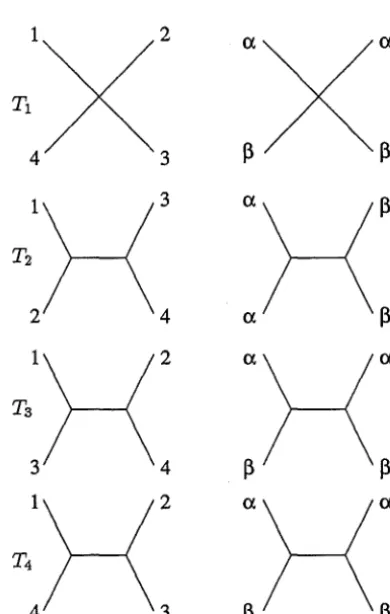
Definitions 1 (Phylogenetic trees, characters) A phylogenetic tree is a tree T = (V(T), E(T)) having no vertices of degree two and such that each leaf ( degree one vertex) is given a unique label from { 1, ... , n}, where n is the number of leaves of T. We say that T is a tree on n leaves, and write

[n]

for

{1, ... , n}. Where convenient, we identify each leaf with its label. If every

in-ternal (non-leaf) vertex of T has degree three, we say that T is binary. In the case of rooted trees, we allow the root to have degree two.

A function

x :

[n) 1-+ G, where G is a set of r colours, is an (r-colour)

lx2

T1

4 3

Figure 1: Some examples of phylogenetic trees.

called a colouration of T; if

x is such that xl[n]

=

x

(that is x agrees with

x

on the leaves of T) then

x

is called an extension of

x (

on T ).

Notation: The edge incident with the vertices u and v will usually be denoted by { u, v }. However, where we consider this edge to be directed from u to v it will be denoted by the ordered pair (

u, v).

Figure 1 shows the four (unrooted) phylogenetic trees on four leaves and the way in which the binary character

2 3

(1)

f3

[image:4.603.122.317.135.442.2]

(T,X)

>--<~

ex

ch(x)=2

ch(x)=3

ch(x)=3

ch(x)=2

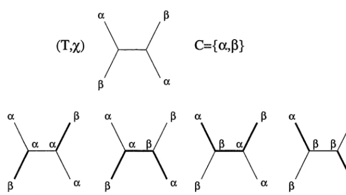
Figure 2: To find f(x, T) for the tree and character shown with colour set C

=

{ex,

.B},

consider all possible colourations of the internal vertices. Since T has two internal vertices, there are 22

=

_{4 such colourations. Bi-coloured edges} are shown bolded. The minimum value of ch(x) is two, so that f(x, T)

=

2. _ There are two minimal extensions.

With each character

x

and phylogenetic tree T on n leaves we may associate a non-negative integer (the "length" of

x

on T) as follows.

Definitions 2 (length of

x

on T, minimal extensions) If

x :

V(T) 1-t C

then the changing number of

x,

ch(x), is the number of edges e

= {

u, v} such that x( u)

=f.

x( v). Such an edge is said to be bi-coloured.

If

x :

[n] 1-t C then the length of

x

on the phylogenetic tree T,

f(x,

T), is the

minimum of ch(x) over all extensions x of

x

on T. An extension of minimal changing number is called a minimal extension of

x

(on

T).

Biologically, we interpret each vertex of a phylogenetic tree as representing a species, with the edges denoting (immediate) ancestor-descendant relationships. The leaves represent extant species, the internal vertices ancestral species, and in rooted trees the root represents a common ancestral species from which all other species on the tree are descended. Since we are primarily interested in speciation events, where the tree "branches", we do not allow vertices of degree two except possibly at the root.

[image:5.618.101.451.133.330.2]

a

(ii)

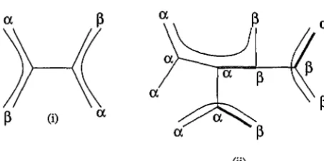
Figure 3: Some path systems illustrating Menger's theorem. (i) A maximal path system for the tree and character in figure 2.

(ii)

A set of three edge-disjoint paths joining differently coloured leaves, together with an extension of changing number three. By Menger's theorem the character shown has length three on the given tree.

therefore the minimum number of mutations required for it to evolve on the tree, and is used in methods such as maximum parsimony to estimate the true phylogeny of extant species.

-2.2

Menger's theorem and Erdos-Szekely path systems

In practical applications the length of a character on a given tree is found using Fitch's algorithm, which is an order n process for determining l(x, T) and finding a minimal extension. However, for theoretical purposes l(x, T) is usefully given by Menger's theorem and Erdos-Szekely path systems, two results that will be of great importance to us in later sections. We state them here in the form in which we will be using them, rather than in their full generality.

Theorem 1 (Menger's theorem for trees, [1]) If

x

is a binary character then

.e(x,

T) equals the maximum number of edge-disjoint paths connecting dif-ferently coloured leaves of T.

Although Menger's theorem applies only to binary characters, an extension to r-colour characters has been developed recently by Erdos and Szekely [5].

Definitions 3 (Erdos-Szekely path systems) An Erdos-Szekely path sys-tem for

x

on T is a set 'P of directed paths in T satisfying the following condi-tions:

1. Each path joins leaves coloured differently by

x.

2. If two paths use the same edge of T, then

[image:6.602.106.333.132.245.2]

(b) they are directed towards leaves coloured differently by X·

If 'P has the maximum cardinality of any Erdos-Szekely path system for

x

on T, then 'P is said to be optimal.

Notation: Following Erdos and Szekely [5] we denote the starting vertex of a directed path P by s(P) and the terminal vertex of P by t(P).

Theorem 2 (Erdos and Szekely [5]) The size of an optimal Erdos-Szekely

path system for

x

on T equals

.e(x,

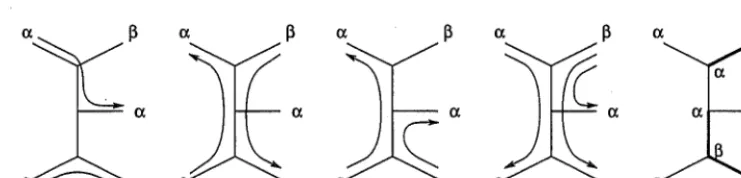
T).

Figure 4: Some path systems and a colouration illustrating Erdos-Szekely path systems and Theorem 2. (i)-(iv) show some path systems, of which only (iv) is an Erdos-Szekely path system. (v) shows a minimal colouration.

Figure 4 illustrates Erdos-Szekely path systems and Theorem 2. Only one of the path systems shown is an Erdos-Szekely path system: (i) contains a path connecting leaves that are the same colour a, violating condition 1; in (ii) each path joins differently coloured leaves, but the same edge is used in opposite directions by two paths, breaking condition 2(a); while in (iii) condition 2(a) is satisfied but 2(b) is not as both paths share an edge and are directed towards identically coloured leaves. (iv) is an Erdos-Szekely path system since all of the conditions are satisfied. The colouration in (v) has changing number three, and it follows from Theorem 2 that the path system in (iv) is optimal and that the character has length three on the given tree.

Note that although Theorem 2 includes the case r

=

2, it does not reduce to Menger's theorem when

x

is binary, as it allows the paths to intersect. Viewed in the light of Theorem 2, Menger's theorem guarantees us the existence of an edge-disjoint Erdos-Szekely path system when r

=

2, a fact we will make use of in section 4.

2.3 A Markovian model of character evolution

The model we will be considering is a generalisation to r colours of the Cavender-Farris (two colour case, [3, 6]) and Jukes-Cantor (four colour case, [10]) models.

[image:7.618.92.463.277.366.2]

Given a rooted phylogenetic tree T, a probability distribution 1r of colours at the

root p and a mutation probability Pe on each edge e of T, the colour at the root "evolves" down the tree, assigning a colour to each vertex of T and generating a colouration

x

of T. We suppose that this evolution takes place such that

• there is a total order

:S

of the vertices, respecting ancestry (so u

<

v if u is nearer the root than v is), such that

P[x( v)

=

al /\

x( w )]

=

P[x( v)

=

a:ix( wo)] Va: E C, v E V(T) (2)

w<v

where w₀ is the immediate ancestor of v

• the probability of a net change of colour occurring across an edge e is given by Pe, and if a net change occurs, each of the remaining r - 1 colours is equally likely

• Pe satisfies

O

:S

Pe

:S

(r -

1)/r.

The probability of generating a given colouration

x

will in general depend on T, 1r and the vector p

=

(Pe)eeE(T) of probabilities and is given by

P[xlT,

1r,p]

=

1r(x(p))

II

(1-Pe)

II

e={u,v}:

x(u)=x(v) x(u):;cx(v) e={u,v}:

(3)

The probability of generating a character

x

under the model is found by summing (3) over all extensions

x

of X, so that

P[xlT,

1r,p]

=

I:

P[xlT,

1r,p] .

(4)

x:x1t ..

1=x

Figure 5 shows a calculation of P[xlT, 1r, p] for a simple tree and character.

The origin of the upper bound of

(r -1)/r

on Pe lies in the assumption that changes of colour along an edge take place under a continuous-time Markov process. This generates a mutation probability Pe-the probability of a net change across the edge-such that O <Pe<

(r-1)/r,

depending on the "length" of the edge; for simplicity we include the endpoints so that our set of possible vectors is compact. The mutation probabilities thus give some indication of the relative lengths of time along each edge, with Pe tending to (r -

1)/r

as the "length" of e increases.

In a more general setting, we might allow each edge to be governed by an r x r transition matrix me whose a:/3-entry gives the probability that a change from a to

/3

occurs across e, given that the vertex nearer the root is coloured

a. Under this model, (2) implies

II

e

mx(u)x(v) . (5)

p,1t

~

2 3

X(i) a

1 2 3

P[xlT,

1r,p]

=

1r(a)(l - P1)(l - P2)(l -

p3)p4

( l

~

( l ( l ~

~

(l ( l ~

~

(l ( l ~

=

P[xlT,

1r,p]

Figure 5: To calculate P[xlT,

1r,p]

for the tree and character shown, sum

IP'[xlT,

1r,p]

over all extensions

x

of X· In the two colour case, each bi-coloured edge contributes a factor of Pe to IP'[xlT,

1r,p];

all other edges contribute a factor of 1-Pe·

Note that in this case the product is taken over edges directed away from the root, as the matrices need not be symmetric. For our model the transition matrices are

(

1 _{- Pe} -2.L _r-1

me=

~

1-pe

-2.L

r-1 -2.L r-1

Each diagonal entry is 1 - Pe and all the off-diagonal entries are Pe/(r - 1).

2.3.1 Mutation probability along a path

(6)

Our first result is a generalisation to r colours of a result due to Hendy [9] in the two colour case.

8

[image:9.618.96.414.129.386.2]

Lemma 1 (Mutation probability along a path) If u and v are vertices of T, then

P[x(u) =fa x(v)IT, 1r,p]

=

r - l (1- IT(l - _!__lPe)),

r r

-eeP

(7)

where P is the path between u and v.

Proof: The result may be proved by induction on the length of the path or using linear algebra. We give the linear algebra proof.

If u is an ancestor vertex of v then the transition matrix mp for the path is the product of the matrices me along the path. Diagonalising the matrix in (6)

we find

me= Hdiag(l, 1-~Pe,.,., 1-~Pe)H-1,

r - r - (8)

where

1 1 1 1 1

1 -1 1 1 1

1 0 -2 1 1

H=

1 0 0 -3 (9)

1

1 0 0 0 1-r

Hence

mp

=

H diag(l, IT (1 -

r:

1 Pe), ... , IT (1-

r:

1

Pe))H-1_,

(10)

eEP eeP

which by (8) is a matrix of the form in (6) with mutation probability

r-1 IT r

PP= - ( 1 - (1-

-pe)).

r r - l

eeP

(11)

Now if u and v are arbitrary vertices of T, let w be their most recent common ancestor, 7rw the distribution of colours at w and P1, P2 the path mutation

probabilities from w to u and v respectively (see figure 6). The probability that u and v are the same colour is

P[x( U)

=

x( V)

IT,

71", p]

=

L

[1rw ( a )(1 - P1)(l - P2)

+

L

1rw (

"Y)

(rp~p:)2]

aec ~ec

(1-P1)(l - P2)

+

PlP2 r - l r

= 1 - P1 - P2

+

--P1P2, r - l

p

•

I I I I I I

,' w,1rw

P1,iA~·P2

u v

Figure 6: If u and v are not related by direct descent, break P as shown into the paths

Pi

and P2 with associated path mutation probabilities P1, P2, where w is the most recent common ancestor of u and v.

since each 1r w ( _{1 ) appears} r-1 times in the sum over a and 1 , and I::Cl'eC 1r w (a)

=

1.

Therefore

P[x(u)

=J

x(v)IT, 1r,p]

r Pl

+

P2 - r _ l P1P2

r-l r r

=

-r-(l - (1 - r - 1 P1)(l - r - 1 P2)) (12)

and substituting Pi

=

r;1 (1 - Ileep/1 - r:₁Pe)) from (11) for each i we ob-tain (7).

Remark: Note that if u and v are not related by direct descent then the transition matrix for the path P is not necessarily of the form in (6). However, in the case of an even distribution of colours at the root it is easily checked that we do obtain such a matrix.

2.3.2 Dealing with the root

The presence of the root and the distribution 1r introduce complications we would rather be without. Most tree reconstruction methods return unrooted trees, so that the position of the root is generally not known. The distribution at the root is typically another unknown. We consider here two ways of obtaining some measure of

P[xlT]

on an unrooted tree closely related to T.

Firstly and most simply we could assume an even distribution of colours at the root, that is 1r(a)

=

l/r \/a EC, to get

1

P[xlT, 1r,p]

=;:

L

II

(1-Pe)

II

x:xl( .. 1=x e={u,v}: e={u,v}: x(u)=x(v) x(u);cx(v)

Pe

[image:11.618.184.474.66.272.2]

This expression is independent of the location of the root so we may treat the tree as unrooted. Where the root has degree two this does not give us an unrooted phylogenetic tree since we do not allow non-root vertices to have degree two, but in this case we may use the remark following Lemma 1 to collapse the root and the two edges incident with it to a single edge with the path mutation probability

r-1 r r

PP = - ( 1 - (1 - -p1)(l - -p2)),

r r-1 r-1 (14)

thereby obtaining an unrooted phylogenetic tree (see figure 7).

Figure 7: Deleting the root. The circles marked T1, T2 denote rooted subtrees.

A second approach is to allow a transitive subgroup G of Sc, the symmetric group on C, to act naturally on the set of characters on n leaves according to

(O'X)(i)

=

O'(X(i)) 'iO" E G, i E [n]. Summing over an orbit Gx we have

- IP'[GxlT, 1r,p]

=

L L

IP'[xlT, 1r,p]

uEG x:xhn1=ux

L L

1r(x(p))

IT

(1-Pe)

IT

uEG ;x:xhnJ=ux e:::{u,v}: e:::{u,v}: x(u)=x(v) x(u)#x(v)

Pe

r-1

If

x

is an extension of x then O"X. is an extension of O"X, so we may exchange the order of summation to get

P[GxlT, 1r,p]

=

I:

1r(O'x(p))

II

(1 - Pe)

IT

e:::{u,v}: e={u,v}: ux(u):::ux(v) ux(u)#x(v)

Pe

r-1

(1-Pe)

IT

r

~

1

L

1r(O''f<.(p)) '

x:xhn1=X e={u,v}:

II

e={u,v}: uEG x(u)=x(v) x(u)tx(v)

the last following from O"X.( u)

=

O"X.( v) if and only if x( u)

=

x.( v). Finally, G is transitive and Laec 1r(a)

=

1 so that LueG 1r(O'X.(P))

=

IGl/r, and

IT

IGI ~

P[GxlT, 1r,p] =

7

L;

x:xi( .. 1=x e={u,v}: x(u)=x(v)

(1 - Pe)

IT

e={u,v}: x(u)tx(v)

Pe

[image:12.602.116.444.391.458.2]

Thus P[GxlT, 7r,p] is independent of 7r and we have an expression very similar to that in (13) where we considered the even distribution case. Where the root has degree two we may again collapse it and its incident edges as in figure 7 to obtain an unrooted tree with P[GxlT, 7r,p] unchanged.

Where G

=

Sc we note that Gx is the set of all characters inducing the partition {x-1_{({a}): a EC} of [n].}

Both of the above methods allow us to associate an unrooted tree with each rooted tree. Where the root has degree greater than two, the unrooted tree is identical to the rooted tree except that we no longer distinguish the root; where the root has degree two we collapse the two edges incident with it to a single edge. The mutation probability across this edge is the net mutation probability across the path formed by the two collapsed edges. The sum over extensions of xis common to both (13) and (15), motivating the following definition::

Definitions 4 For an r-colour character

x

and an unrooted tree T we define

P'[xlT,p] =

I: II

x:xi(,,1=x e={u,v}: x(u)=x(v)

(1-Pe)

II

e={u,v}: x(u);cx(v)

_1?.!_

r - l (16)

In the case of an even distribution of colours at the root P'[x, T,p] may be interpreted as the conditional probability of generating

x

on the rooted tree from which T was obtained, given that leaf 1 (say) is coloured x(l). This follows from (13) and the fact that an even distribution of colours at the root induces an even distribution of colours at each leaf.

For much of the remainder of this discussion we consider P'[xlT,p] and un-rooted trees.

3 Bounding

r'[xlT,p]

Penny et. al. [11] have shown that in the two colour case,

max{IP''[xlT,p]}

=

2-t(x,T). p

A major result of this project is an extension of this result to r colours:

(17)

Theorem 3 (Upper bound for P'[xlT, p]) If

x

is an r-colour character and T is an unrooted tree, then

max{IP''[xlT,p]}

=

r-t(x,T). p

As a corollary to the proof of Theorem 3 we have the following:

Theorem 4 A minimal extension of an r-colour character

x

on T is uniquely determined by X and the set of edges it bi-colours. That is, if X1 and X2 are minimal extensions of X and

{e

=

{u,v} E E(T): x1(u)

#

x1(v)}

=

{e

=

{u,v} E E(T): x2(u)

#

x2(v)},

(19)

then x1

=

X2·

Before proving Theorem 3 we consider the proof in the two colour case. If Pis a path in T joining leaves i and j, put

</J(P) _ { 1 if x(i)

#

x(j)

-

o

if

x(

i)

=

xU) ·

(20)

By Menger's theorem there is a set

{Pi, ... ,

Pt} off, edge-disjoint paths such that efJ(Pi)

=

1 for i

=

1, ... , £, and by Lemma 1

1 1

P[efJ(P)

=

llT,p] =pp=

2

(1-

II

(1- 2pe)) ~

2

.

(21)

eEP;

Our first two assumptions on page 7 imply that changes of colour on different edges are independent, so that the </J(Pi) are independent variables since the Pi are edge disjoint. Hence

P[</J(P1)

=

1, ... , </J(Pt)

=

llT,p]

l

IlP[efJ(Pi)

=

llT,p]

i=l

<

rt

'

implying P'[xlT, p] ~ 2-t. To complete the proof, a vector p such that P'[xlT, p]

=

2-t is exhibited.

The strong use of Menger's theorem, in the requirement that the paths be edge disjoint, effectively prevents any natural extension of this proof tor colours as an optimal Erdos-Szekely path system may have intersecting paths.

3.1 Proof of Theorems 3 and 4

We begin by reducing to the case where Pe is either O or ( r - 1) / r for every edge e of T. For notational convenience put

M(T)

=

{p E [O, (r - 1)/r]IE(T)I : Pe E {O, (r - 1)/r }Ve E E(T)} (22)

and define

E(p)

=

{e E E(T): Pe= (r - 1)/r} for each p E M(T), and

E(x) = { e

= {

u, v} E E(T) : x( u)

#

x( v)}

. (23)

(the change set or bi-coloured set of x) for each colouration

x

of T.

Let

x

be an r-colour character of length £ on an unrooted tree T. For this section we consider x and T to be fixed and write P'(p) for P'[xlT,p], to emphasise the view of P''[xlT, p] as a function of p. Thus

P'(p)

=

I:

IT

x:xl( .. 1=x e={u,v}:

x(u)=x(v)

(1 - Pe)

IT

e={u,v}: x(u);cx(v)

Pe

r - l (25)

Note that for each edge e of T, Pe occurs in each term in the sum in (25) exactly once. Let p E [O, (r - 1)/r]IE(T)I. Choosing e' E E(T) and fixing Pe for e E E(T) \ {

e'}

(so that we regard P(p) as a function of Pe'), we therefore obtain a polynomial of degree at most one in Pe'. On a closed interval, the extreme values of ~uch a polynomial occur at the end points, so there is a vector p' of mutation probabilities such that

, { Pe if e

#-

e'

Pe

=

0 or r~l if e

=

e' (26)

and

P(p)

:s;

P(p'). (27)

Carrying out this process for each edge of T in turn, we eventually arrive at a -vector p" such that p" E M(T) and

P(p)

:s;

P(p").

We have established the following lemma:

Lemma 2 maxp{P'[xlT,p]} is realised by some p E M(T).

Now let p E M(T). Each extension

x

of

x

contributes a term

P'[xlT,p] =

IT

(1-Pe)

IT

e={u,v}: x(u)=x(v)

e={u,v}:

x<

u );ex( v) Pe r - l

(28)

(29)

to P(p). If there is an edge

e

= {

u,

v} for which x(

u)

#-

x(

v)

and Pe

=

0, then a factor of zero occurs in the right-hand product in (29) and we have P'[xlT, p]

=

0.

Hence we need only sum over extensions x such that E(x) ~ E(p). Further, if E(x) ~ E(p ), then each edge e

= {

u, v} contributes a factor

{

!=I

=

f

if x(u)

#-

x(v)

mi(u)x(v)

= ·

1- Pe=

f

if x(u)

=

x(v) and Pe= r;l

1 - Pe

=

1 if x( u)

=

.x( v) and Pe

=

0

(30)

Lemma 3 If p E M(T), then

P(p)

=

rlE~v)l

l{x: Xi[nJ

=

X, E(x)

~

E(p)}I.

(31)

By Lemma 3, to calculate P(p) for p E M(T), we must count the number of extensions x of

x

for which E(x) ~ E(p). With a view to proving Theorem 3, we would like to show that

l{x: Xl[n]

= X, E(x) ~ E(p)}I ~ rlE(p)l-t, (32)

with this bound attained by some p E M(T). Since it may be the case that there are no extensions with E(x) ~ E(p) (this will certainly be the case if

IE(p)I

<

.e),

we make the following definition:

Definitions 5 (x-viable) S ~ E(T) is x-viable or viable for

x

on T if there is an extension

X

of

x

such that E(x) ~ S.

Let S be viable for X on T,

X

such that E(x) ~ S, and put k =

ISi.

Deleting S from T, which we denote by T\S, will divide Tinto k+ 1 connected components, and

X

must be constant on each of these since E(x) ~ S. In _particular, if v is a vertex belonging to a component containing a leaf i of T, then we must have x( v)

=

x(

i).

However, on components that do not contain a leaf of T,

X

may take any of the r colours in C. Since xis completely determined by the colour of each connected component of T \ S, it follows that if there are

>.

components not containing a leaf of T then there are precisely

r>-

extensions of

x

such that E(x) ~ S.

Definitions 6 (internal and external components) If S ~ E(T), a con-nected component of T \ S that does not contain a leaf of T is an internal component. A connected component that does contain a leaf of T is an external component.

Figure 8 shows an example of a tree and character with a set of x-viable edges deleted. The deleted edges are shown as dashed lines and the connected com-ponents are circled. There is one internal component.

The inequality (32) follows from the above arguments and the following theorem:

Theorem 5 Let

x

be an r-colour character of length .e on T. If S is viable for X on T and

ISi

=

k, then T \ S has at most k - .e internal components.

Proof: Let P

=

{P1 , ... , Pt} be an optimal Erdos-Szekely path system for

x

[image:17.618.102.249.137.260.2]

a

... ,····

Figure 8: An example of T \ S.

define f : 'P 1-+ E(T) by f(P)

=

e if e is the last edge in S on P. The

conditions for an Erdos-Szekely path system then imply that

f

is one-to-one. For if f(Pi)

=

f(PJ)

=

e

= (

u, v), then both Pi and Pj must use e in the direction from u to v, and since no edges in S lie on that part of Pi from v to t(Pi), nor on that part of Pj from v to t(PJ ), t(Pi) and t(PJ) belong to the same connected component of T\ S. This contradicts the fact that Sis x-viable and x(t(Pi)) =f:. x(t(PJ )) for intersecting paths Pi and Pj of an Erdos-Szekely path .system.

Consider f('P). We have

lf('P)I

=

£ since f is one-to-one and

IPI

=

£, so that T \ f

('P)

has £ + 1 connected components. We show that each component of T \ f('P) contains a leaf of T. When the remaining edges in S are deleted, there will still be at least£+ 1 connected components containing a leaf of T, so that T \ S has at most k + 1 - (£

+

1)

=

k - £ internal components.

Let v E V (T). The connected component of v in T \

f

('P)

will contain a leaf of T if there is a walk from v to a leaf that does not cross an edge of f('P). Let W be a walk from v to any leaf of T. If W does not cross any edges in f('P) we are done; otherwise there is some Pi E 'P such that f(Pi)

=

ei

=

(ui, Vi) is the first edge in f('P) that W crosses. We consider two cases, according to the direction in which W crosses ei.

If W crosses ei in the opposite direction to Pi (so that W arrives at Vi before ui), then since ei is the last edge in f('P) on Pi, the path W' formed by following W as far as Vi and then traversing Pi forwards from Vi is a path from v to the leaf t(Pi) that does not cross any edges in f('P) (see figure 9).

Figure 9: The walk W from v crosses f(Pi) in the opposite direction to Pi, Trace Pi forwards to t(Pi) to obtain W'.

W' as far as Vj and then tracing Pj forwards to t(Pj) joins v to a leaf without crossing any edges in f(P) (see figure 10).

•

w /

I

I I I

I

•

'

'

'

~:::==::::---,, Vi ' '

Uj':~~~~

I I

I

/ P·

• J

s(P1)

'

_'

'

_' [image:18.602.214.329.142.250.2]

pi '•

Figure 10: The walk W from v arrives at Ui before Vi, Retrace Pi towards s(Pi) to form W'. If W' arrives at s(Pi) without crossing any edges of f(P) we are done; otherwise, we arrive at Vj and may trace Pj forwards to t(Pj) without crossing any edges of f(P), forming W".

Therefore, given any vertex v of T there is a path joining it to a leaf of T that does not cross any edges in f(P), and we conclude that each connected component of T \ f(P) is external. The result follows.

Theorem 4 follows as an easy consequence of Theorem 5:

[image:18.602.211.437.356.494.2]

Proof: If x 1 is a minimal extension of x then E(x1) is ax-viable set of cardi-nality f(x, T). Then, by Theorem 5, T \ E(x1) has no internal components so that there are exactly r0 = 1 extensions x of x such that E(x) ~ E(xi), namely x

=

Xl· Hence if E(x1)

=

E(X2) then x1

=

X2·

Theorem 5 establishes the inequality (32), proving P'[xlT,p) :::; r-t(x,T). To complete the proof of Theorem 3, we must exhibit a vector of probabilities p such that P(p) = r-t. The vector pX defined by

.

{ r;l

if x(u)

#

x(v)

P{u,v} -X

-O if x(u) = x(v)

(33)

is easily seen to be such a vector whenever

x

is a minimal extension of

x

and we have our result.

3.2

Bounding

P[xlT,

1r,p]

We consider here briefly applying Theorem 3 to the problem of bounding IP[xlT, 1r,p]. For an arbitrary root distribution, we have

P[xlT, 1r,p] :::; max1r(a) P'[xlT,p) aec

<

max1r(a) r-t(x,T).

aeC (34)

This bound will certainly be sharp if there is minimal extension

x

of

x

such that 1r(x(p))

=

maxaec 1r(a). In the special case of an even distribution of colours at the root, we have

P[xlT, ?T, p] :::; r-t(x,T)-1, ₍₃₅₎

with this bound achieved by vectors pX for minimal extensions

X·

4 Realising the upper bound in the two colour

case

Theorem 6 If xis a binary character then p maximises P'[xlT,p] if and only if p

=

pX,

for some minimal extension

x

of X, where

.

{ !

if x(u)

'#

x(v)

PX

_{{ u,v}} = _,

A A

O if x(u)

=

x(v).

(36)

The backward direction of Theorem 6 is already established; we prove the for-ward direction in two stages, first establishing it for binary trees, and then reducing the general case to that where T is binary.

4.1 Proof of Theorem 6 for binary trees

The proof is by induction on n, the number of leaves of T. Consider n = 2, for which there are two possible characters X up to permutation (see figure 11). Clearly P[xlT, p] is maximised in the first case only if Pe

=

0, and in the second

Pe

P'[xlT, p] = 1 - Pe

Pe

/3

IP'[xlT,p] = Pe

Figure 11: The two possible characters when n

=

2.

only if Pe

=

1/2.

Suppose the result is true for binary trees on n - 1 leaves, where n

2:

3. Let T be a binary tree on n leaves,

x

a character of length f on T, and suppose that p is such that P'

[x IT,

p] is maximised. Since T is binary, it has a pair of adjacent pendant edges, that is a pair of edges { u, v} and { u, v'} such that v and v' are leaves of T (see figure 12). We consider two cases: x(v)

=

x(v'), and x(v)

'#

x(v').

Case 1: x(v)

=

x(v'). [image:20.602.218.399.353.483.2]

v

T

1---< u

v'

Figure 12: A tree T with a pair of adjacent pendant edges, { u, v} and { u, v'}. The circle marked

T

denotes. a rooted subtree.

leaves ofT' such that Xa agrees with x on their common leaves and Xa(u) = a, and define Xf3 similarly. For convenience put e

= {

u, v }, e'

= {

u, v'} and let the vertex w and edge e" be as shown in figure 13.

v e e" _u

T e' v'

Figure 13: The trees T, T' and characters Xa, Xf3·

Then

P''[xlT,p]

=

(1-Pe)(l - Pe1 ) P''[xalT',p]

+

PePe' P''[xf31T',p]. (37)

Now if x is a minimal length extension of

x

on T then x(u) = a; for if x( u)

=

a we get no changes on e, e' and e" if x( w)

=

a' and one change if x(w)

=

(3, while if x(u)

=

(3 we get two or three changes depending on whether x(w) equals a or (3. It follows that Xa has length Con T'.

However Xf3 may have length less than £. For if x is an extension of x such that x( u)

=

(3, then xis not a minimal length extension of

x

and so has changing number at least C

+

1. But two of these changes occur on e and e', which are deleted in forming T' and Xf3, so that ch(xlv(T')) ~ C - 1. Hence Xf3 may have length less than C but the decrease is by at most one. (For an example showing that this can in fact occur, see figure 14). [image:21.618.216.345.144.200.2] [image:21.618.103.336.306.453.2]

Figure 14: f(Xf3, T') f(Xf3, T')

=

1.

a

a

a

(T,x)

frp

~

~

a

~

may be less than f(x, T). Here

=

rt((l - Pe)(l - Pe')+ 2PePe')

= 2-\1 - Pe - Pe'

+

3PePe1 ).

~

f(x,T)

=

Consider 1- Pe - Pe'+ 3PePe'

=

1 - Pe'+ Pe(3Pe' - 1). If Pe= 0 then

1 - Pe - Pe1

+

3PePe1 = 1 - Pe'

S

1,

2 but

(38)

with equality if and only if Pe' = O. If Pe

>

0 and O:::; Pe'

<

1/3 then Pe(3Pe' -1)

<

0 so l-pe-Pe' +3PePe'

<

1. Finally, if 1/3

S

Pe'

S

1/2 then l-Pe'

S

2/3 _and Pe(3Pe' - 1)

S

1/4 so that

2 1 11 1 - Pe - Pe'

+

3PePe1

S

3 + 4

= 12

<

1.

(39)

Hence 1 - Pe - Pe'

+

3PePe'

S

1 with equality if and only if Pe

=

Pe'

=

0.

Since maxp{P'[xlT,p]}

=

2-t and p maximises P'[xlT,p], we must have Pe

=

Pe'

=

0. By the induction hypothesis, IP''[xa IT', p]

=

2-t if and only if p

=

pX,"'

on T' for a minimal extension Xa of Xa· A minimal extension of Xa extends naturally to a minimal extension of x and Pe

=

Pe'

=

0 so that p

=

pX for a minimal extension

x

of X on T.

Case 2: x(v) :j:. x(v').

Without loss of generality x( v)

=

a and x( v')

=

/3.

Let T', Xa and X{3 again be as in figure 13. If

x

is a minimal extension of

x

then

x

involves a change on exactly one of e, e' regardless of the colour assigned to u, so that f(Xa, T'), f(Xf3, T') ~ f- 1. Hence

IP'[xlT,p]

=

(1-Pe)Pe' IP''[xalT',p]

+

Pe(l - Pe1 ) P'[Xf31T',p]

S

rt+

1

((l -

Pe)Pe'

+

Pe(l - Pe1 ))

=

rt(l - (1 - 2pe)(l - 2Pe' )). ( 40) [image:22.602.106.458.111.515.2]

(i) Pe= 0, Pe'= 1/2 and P'[xalT',p] = 2-£+1; (ii) Pe

=

1/2, Pe'

=

0 and P'[x.6

IT',

p]

=

2'""l+1;

or if PePe' =I= 0 then

(iii)

P'[xalT',p]

=

P'[X,61T',p]

=

2-l+l and at least one of Pe,Pe'

=

1/2.

Under the induction hypothesis (i) and (ii) have p

=

pX,

for a minimal extension

X,

so it remains to show that (iii) cannot occur. By the induction hypothesis, P''[xalT',p]

=

P''[xf31T',p]

=

2-t+i occurs if and only if E(p)

=

E(xa)

=

E(X,6) for minimal extensions Xa and X/3 of Xa and X,6 respectively. Let i be a leaf of T' other than u, and without loss of generality assume x(i)

=

a. Consider the number of changes that occur on the path P from i to u. Since Xa(i)

=

Xa(u) an even number of changes must take place on this path under Xai but X/J(i) =I=

X,6(u) so that an odd number of changes must take place under X/3· Hence E(xa)

=

E(X/3) is not possible, so that (iii) cannot occur and the theorem is proved for binary trees.

4.2 Splits and refinement

In this section we introduce some concepts required for an auxiliary theorem (Theorem 9) that will allow us to reduce the general case to the case just proved.

-Definitions 7 (Splits) A split is a bi-partition of[n].

Splits arise naturally from trees and are a convenient method of comparing and dealing with trees. Given an edge e ofT, we obtain a split corresponding to e by deleting e and grouping the leaves in each of the rooted subtrees thereby created (see figure 15). Doing this for each edge of T we obtain the set of splits of T, O'(T). The following theorem (Buneman, [2]) shows that O'(T) contains all the information contained in T:

Theorem 7 A set :E of splits is O'(T) for a phylogenetic tree T if and only if

1. {{i}, [n) \ {i}} E :E, i = 1, ... ,

n;

2. For each pair {A, B}, {C, D} E :E, at least one of An C, An D, B n C and B

n

D is empty.

Furthermore, O'(T)

=

O'(T') if and only if T

=

T'.

A set of splits satisfying condition (2) above is said to be pairwise compatible. Splits may be used to define a partial order on the set of trees on n leaves:

Theorem 8 The order :$ defined by

(41)

[image:24.602.198.442.148.271.2]

Figure 15: An edge and its corresponding split. Deleting the edge e from T, we obtain the split { {1, 2, 3, 4}, {5, 6, 7, 8}}.

Definitions 8 (Refinement) If T1 ~ T2 then T2 is said

to

be a refinement of T1,

We may now state and prove the theorem required for the reduction of Theorem 6 to the binary tree case.

Theorem 9 Let T be a tree and

x

a binary character. There is a binary tree T' refining T such that £(x, T') = £(x, T). T' may be chosen in such a way that the minimal extensions of

x

on T' are in a natural bijective correspondence with the minimal extensions of

x

on T.

Proof: Let P be a set of£

=

£(x, T) edge-disjoint paths joining differently coloured leaves, the existence of which is guaranteed by Menger's theorem. Form the sequence T

=

T1

<

T2

< · · ·

refining T inductively as follows. Given

11,

choose v E V(11) of degree greater than or equal to four. If there is a path P E P passing through v, choose e1 and e2 incident with v and lying

on P; otherwise choose e1 and e2 incident with v arbitrarily. If _{e 1 ,...,} {A, B},

e2 ,..., { C, D} and

An

C

=

0,

it is easily checked that

{AU

C, B

n

D} is a split and that

E

=

<7(11) U {{AU

C, B

n

D}} is pairwise compatible, so we may put

<7(11+1)

=

E. Then 11

<

11+1,

and no path in Plies on the edge corresponding to

{AU

C, B

n

D} so that P remains edge disjoint in

11+1

(see figure 16).

The new edge in

11+1

splits v into two vertices, one of degree three and one of degree one less than that of v, so this process must eventually terminate in a binary tree Tm

=

T'. P remains edge-disjoint in T' so by Menger's theorem we have £(x, T')

2:

£. If xis a minimal extension of x on T then we may obtain an extension

x

of

x

on T' by identifying each vertex of T' with the vertex of

'

'

11+1

Figure 16: The refinement process. The splits are shown by dotted lines. None of the paths in P lie on the new edge of 11+1, so that P remains edge disjoint in 11+1 · v splits into two vertices, one of degree three and the other of degree one less than the degree of v.

corresponds to a split of T and the corresponding edge of T is bi-coloured, so that ch(x)

=

ch(x)

=

f, implying f(x, T') ~ f and hence equality.

Furthermore, every minimal extension of

x

on T' arises in this way. Let

x

be such an extension. Since each path in P joins differently coloured leaves, there must be at least one change on each path. Moreover, P has cardinality f(x, T'), so there is exactly one change on each path and no changes on edges _not on paths. Since none of the newly created edges lie on any of the paths,

X

must be constant on the set of vertices identified with a given vertex v of T, and we obtain a minimal extension

x

of

x

on T by putting

x(

v) equal to this common colour.

4.3 The general case of Theorem 6

We now complete the proof of Theorem 6 in the general case.

Let T be a phylogenetic tree,

x

a binary character and suppose p maximises P''[xlT,p]. Let T' be a binary tree refining T as constructed in Theorem 9, and put p~, = Pe if e and e' correspond to the same split <T of T, and p~, = 0 if e'

does not correspond to a split of T. Then

P''[xlT',p']

=

I: IT (

1 - p~)

IT

p~.

x:xl1n1=x e={u,v}: x(u)=x(v)

e={u,v}: x(u);cx(v)

(42)

On newly created edges of

T',

p~ = 0 so we need only sum over extensions for which no changes occur on newly created edges. Such an extension corresponds to an extension of

x

on T, and it follows that

P'[xlT',p']

=

P'[xlT,p]

=

r.e(x,T)

=

r.e(x,T'). (43) [image:25.618.104.337.135.236.2]

of

x

on T', and it follows from the construction of T' that p

=

pX

for a minimal extension

x

of

x

on T.

4.4 Counter-examples for

r

2::

3

Theorem 6 is not true when r

2::

3 even for binary trees, as the following counter-examples show. In part, this appears to be because r may be greater than or equal to the maximum degree of the internal vertices of T, making it easy to create an internal component from E(x),

X

a minimal extension of

x,

by deleting a single additional edge. Since phylogenetic trees are assumed to have no vertices of degree two, this does not occur for binary characters. However, if this requirement is dropped then Theorem 6 no longer holds. In particular, Theorem 6 does not carry over to rooted trees without some modification, as we allow the root to have degree two. We consider this case in section 4.5.

Pe

(T, x) 'Y

Figure 17: A counter-example to Theorem 6 for r = 3.

Example 1: A counter-example to Theorem 6 for r

=

3 is illustrated by the star shaped tree in figure 17. We have f(x, T)

=

2, since ch(x)

=

2 for all three possible extensions of

x

on T. With pas shown, we have:

P'[xlT,p] = (1-p )!! + Pe(l - ~)!+Pe !(l - ~)

e33 2 33 23 3

1 1 1 1

g -

gPe

+

₁₈Pe

+

₁₈Pe

! _

3-2

9 - ' (44)

so that P'[xlT,p] = 3-L(x,T) regardless of the value of Pe·

This example generalises readily to a counter-example for any r

2::

3 by considering the star-shaped tree on r leaves. This is the tree with vertices {O, 1, ... , r} and edges {{O, 1}, {O, 2}, ... , {O, r }}. [image:26.603.220.311.327.439.2]

XJCXX

'Y

(i) 6 (iii)

'Y 6 'Y 6

6 'Y

(ii) (iv)

~---J

I I

I

ct·1

,r' ·· ... ·· ']

(v)

Figure 18: A counter-example to Theorem 6 for r

=

4.

Example 2: A counter-example to Theorem 6 for r

=

4 on a binary tree is illustrated in figure 18. Referring to this figure we have: (i) The tree T and character

x

to be considered.

(ii)

An Erdos-Szekely path system for

x

on T. (iii) A colouration

x

of T of changing number 3. Bi-coloured edges are bolded. The path system in

(ii)

and this colouration, together with Theorem 2 imply t(x, T) = 3. (iv) A set S of edges (bolded). Sis x-viable since E(x) ~ S. (iv) T \ S. Connected components are bolded and edges in S are dotted. There is one internal component (circled), so by Lemma 3 and the arguments following it, if p E M(T) with E(p)

=

S then IP'[xlT,p]

=

4-4_.41

=

_4-3

=

_4-t(x,T).

4.5

Theorem 6 for rooted

trees

In this section we consider the form Theorem 6 takes for rooted trees. We do this only for the even distribution at the root case, as the only case for which the upper bound is sharp.

We have IP[xlT, 1r,p]

=

~ IP'[xlT',p'], where T' and p' are the unrooted tree and mutation probability vector associated with T and p in section 2.3.2, so P[xlT, 1r, p] is maximised if and only if IP''[xlT', p'] is. Where the root has degree greater than two, T

=

T'and p

=

p' so Theorem 6 holds as it stands. If the root has degree two, however, T' and p' are obtained by collapsing the edges incident with the root to a single edge with the path mutation probability

(45)

as in figure 7, section 2.3.2. Vectors p maximising IP'[xlT, 1r,p] are obtained by re-inserting the root as in figure 19 and choosing P1,P2 such that (45) holds.

If pp

=

0 (sop'

=

pX for a minimal extension x of x on T' with x(u)

=

x(

v)

=

a for some a E C) then we must choose P1

=

P2

=

0.

x

may be extended to a minimal extension of X on T by defining

X(P)

= a, and we then have p = pX. [image:27.618.100.410.135.221.2]

minimal extension of X on T by putting either

X(P)

=

a or

X(P)

=

/3,

so in this case we have p

=

pX except on one of the edges { u, p} and { v, p}, on which p . may take any value in the allowed range.

r'::i ..

___!!'__.

.,C"'\

~

_T'

p

~ 2 v

T

Figure 19: Re-inserting the root.

5 Applications to phylogenetic analysis

5.1 Equivalence of maximum parsimony and maximum

likelihood with no common mechanism

Theorem 3 may be used to demonstrate the equivalence of two methods of phylogenetic inference, maximum parsimony and maximum likelihood with no common mechanism. Penny et. al. [11] state this result for the r

=

2 case, and

-a simplified version of their result also appears in Goldman [8]. For a discussion of various methods of phylogenetic inference, see [8].

We consider only the model where the distribution of colours at the root is assumed to be uniform.

Maximum parsimony inference

Given a set X

=

{xi}

of k r-colour characters, choose the unrooted tree or trees T (the "maximum parsimony tree(sr) minimising

k

R(X,T)

=

I:R(Xi,T). (46)

i=l

Interpreting R(Xi, T) as the minimum number of mutations required for Xi to evolve on

T, R(X,

T) is the minimum total number of mutations required for the Xi to evolve on T. Thus maximum parsimony chooses the trees on which the Xi may evolve with as few mutations as possible overall.

Maximum likelihood inference

Definitions 9 (likelihood, Edwards [4]) The likelihood, l[HIR], of the hy-pothesis H given data R and a specific model, is proportional to P[RIH], the constant of proportionality being arbitrary.

A maximum likelihood method of inference chooses the hypothesis H maximis-ing the likelihood function for the data R. For the model under consideration here, we may take the hypothesis to be the tree and mutation probability vector pair (T, p). The maximum likelihood method is then:

Given a set X

=

{xi} of k r-colour characters, choose the unrooted tree and vector pair or pairs (T, p) maximising

k

l[(T,p)IX]

=

P'[XIT,p]

=

II

P'[xilT,p].

(47)

i=l

This is maximum likelihood with a common mechanism, since we require the same vector p to be used for each character; the tree estimated is the "maximum likelihood tree( s )" . If we allow a different vector p for each character ( so that the hypothesis becomes (T, {Pi})) we obtain maximum likelihood with no common mechanism:

Given a set X

=

{Xi} of k r-colour characters, choose the unrooted tree and vector set pair or pairs (T, {Pi}) maximising

k

L[(T, {pi})IX] = IP'[XIT, {Pi}]=

IIP'[xdT,Pt],

(48)

i=l

For the model considered here where we assume an even distribution of colours at the root, we have the following result:

Theorem 10 Maximum parsimony and maximum likelihood with no common mechanism are equivalent, in the sense that both choose the same tree or trees.

Proof: The proof is the same as for the r

=

2 case since it follows directly from Theorem 3. On any given tree

T

we have maxp

P'[xilT,p]

=

r-l(x;,T) so that

k k

max l[(T, {Pi} )IX]=

II

r-t(x;,T) = r-E,=1£(x,,T) = r-l(X,T), (49)

{p;} i=l

and therefore the maximum likelihood trees are precisely the maximum parsi-mony trees.

5.2

The maximum likelihood point is not unique

unique stationary point. Steel [13] gave a simple counter-example to this claim, using a tree on four leaves for which the likelihood function had two extrema at widely separated points. The results of this project show that the likelihood function has more than one stationary point whenever the character considered has more than one minimal extension.

We have seen that

pX,

as defined in equation (33) maximises

P'[xlT,p]

when-ever

x

is a minimal extension of X· By Theorem 4, these vectors are distinct, so that there are at least as many vectors maximising

P'[xlT,p]

as there are minimal extensions of

x

on T (by Theorem 6, exactly as many when r

=

2). Since characters may have more than one minimal extension on a given tree (Steel [12] constructs a tree and character pair with a Fibonacci number of min-imal extensions, see figure 20), it would appear that the likelihood point will in general not be unique.

ex 1 2n-1

)

I I I I

I

1-r(

~ 2 3 4 5 6 7 · · · 2n-2 2n

~ ex ex _{~ ~}

[image:30.600.106.378.304.432.2]

( ') _ { o: if i

=

0, 1 (mod 4), X i -

/3

otherwise.

Figure 20: The tree and character pair shown has a number of minimal exten-sions equal to the nth Fibonacci number.

6 Discussion

The main results of this project are the generalisation of the upper bound on P'[x

IT,

p] from two to

r

colours (Theorem 3) and the complete characterisation of the vectors maximising P'[x

IT,

p] when r

=

2 (Theorem 6). These results answer the two main questions that formed the starting point of this investigation. Of additional interest are the characterisation of minimal extensions in terms of their bi-coloured sets (Theorem 4) and the existence of a binary tree refining a given tree on which a given character has the same length (Theorem 9). This latter result in particular may have applications outside the immediate sphere of interest.

Further work on this model could address the form Theorem 6 should take when r ~ 3 and examine in greater detail the effect of the distribution of colours at the root.

i

7

Acknowledgements

I would like to thank Dr Steel for his supervision of this project.

References

[1] J. A. Bondy and U.S. R. Murty. Graph Theory with Applications. Macmil-lan Press, London, 1976.

[2] P. Buneman. The recovery of trees from measures of dissimilarity. In F. R. Hodson, D. G. Kendall, and P. Tautu, editors, Mathematics in the archaeological and historical sciences, pages 387-395. Edinburgh University Press, 1971.

[3] J. A. Cavender. Taxonomy with confidence. Mathematical Biosciences, 40:270-280, 1978.

[4] A. W. F. Edwards. Likelihood. Cambridge University Press, Cambridge, 1972.

[5] P. L. Erdos and L.A. Szekely. On weighted multiway cuts in trees. Math-ematical Programming, 65:93-105, 1994.

[6] J. S. Farris. A probability model for inferring evolutionary trees. Systematic Zoology, 22:250-256, 1973.

[7] K. Fukami and Y. Tateno. On the maximum likelihood method for esti-mating molecular trees: Uniqueness of the likelihood point. J. Mol. Evol., 28:460-464, 1989.

[8] N. Goldman. Maximum likelihood inference of phylogenetic trees, with special reference to a Poisson process model of DNA substitution and to parsimony analyses. Systematic Zoology, 39( 4):345-361, 1990.

[9] M. D. Hendy. A combinatorial description of the closest tree algorithm for finding evolutionary trees. Discrete Mathematics, 96:51-58, 1991.

[10] T. H. Jukes and C. R. Cantor. Evolution of protein molecules. In H. N. Munro, editor, Mammalian protein metabolism, pages 21-132. Academic Press, New York, 1969.

[12] M. A. Steel. Decompositions of leaf-colored binary trees. Advances in Applied Mathematics, 14:1-24, 1993.