Calculation of Thermal Pressure Coefficient of Dense C15H32, C17H36, C18H38 and C19H40 Using pVT Data

(1)

Calculation of Thermal Pressure Coefficient of Dense

C

15

H

32

, C

17

H

36

, C

18

H

38

and C

19

H

40

Using pVT Data

Vahid Moeini*, Abol Ghasem Mahdianfar Department of Chemistry, Payame Noor University, Tehran, Iran

Email: *[email protected]

Received August 31, 2012; revised October 2, 2012; accepted October 15,2012

ABSTRACT

The thermal pressure coefficients in liquid n-Pentadecane (C15), n-Heptadecane (C17), n-octadecane (C18) and n-nonadecane (C19) was measured using pVT data. The measurements were carried out at pressures up to 150 MPa in the temperature range from 293 to 383 K. The experimental results have been used to evaluate various thermophysical properties such as thermal pressure coefficients up to 150 MPa with the use of density and temperature data at various pressures. New parameters of the linear isotherm regularity, the so-called LIR equation of state, are used to calculate of thermal pressure coefficients of n-Pentadecane (C15), n-Heptadecane (C17), n-octadecane (C18) and n-nonadecane (C19) dense fluids. In this paper, temperature dependency of linear isotherm regularity parameters in the form of a first order has been developed to second and third order and their temperature derivatives of new parameters are used to calculate thermal pressure coefficients. The resulting model predicts accurately thermal pressure coefficients from the lower density limit at the Boyle density at the from triple temperature up to about double the Boyle temperature. The upper density limit appears to be reached at 1.4 times the Boyle density. These problems have led us to try to establish a function for the accurate calculation of the thermal pressure coefficients based on the linear isotherm regularity theory for different fluids.

Keywords: Thermal Pressure Coefficient; Petroleum Industry; Molecular System; The Helmholtz Energy; Lennard-Jones (12,6)

1. Introduction

A study of the thermophysical properties as a function of pressure and temperature in a homologous series of chemical compounds is of great interest not only for indus-trial applications for example, in the petroleum industry, but also for fundamental aspects for understanding the in- fluence of the chain length of the components on the liq-uid structure and then developing models for an accurate representation of the liquid state. With this aim in mind, a research program of thermal pressure coefficients (TPC) measurements under pressure on most paraffins between decane and triacontane was initiated as a part of a project on crude oil characterization [1-3].

One of the most difficult problems within the context of the thermodynamics lies in the shortage for experimental data for some basic quantities such as thermal pressure coefficients (TPC) which are tabulated for extremely nar-row temperature ranges, normally around the ambient temperature for several types of liquids. Furthermore, the measurements of the thermal pressure coefficients made by different researchers often reveal systematic

differ-ences between their estimates [4,5].

The idea has been presented a simple method that use to calculate thermal pressure coefficient directly in place of using equations of state to analysis experimental pVT data [6-8]. The equation of state described in papers is explicit in Helmholtz energy A with the two independ-ent variables density  and T. At a given temperature, the thermal pressure coefficient can be determined by Helmholtz energy [9-15].

Another work has led to try to establish a correlation function for the accurate calculation of the thermal pres-sure coefficients for different fluids over a wide tempera-ture and pressure ranges. The most straightforward way to derive the thermal pressure coefficient is the calculation of thermal pressure coefficient with the use of the princi-ple of corresponding states which covers wide tempera-ture and pressure ranges. The principle of corresponding states calls for the reduced thermal pressure at a given reduced temperature and density to be the same for all fluids. This is true, since the corresponding-states ap-proach is appropriate for conditions of low density in which the fluid molecules are far apart and thus have little interaction. Moreover, at low density, the gas behaves

(2)

ideally and its thermal pressure coefficient is temperature independent and approaches R in the zero-density limit. However, as density increases, molecular interac-tions become increasingly important and the principle of corresponding states fails. The leading term of this corre-lation function is the thermal pressure coefficient of a perfect gas, which each gas obeys in the low density range. Using this condition it can predict the thermal pressure coefficient of different supercritical fluids and refrigerants up to densities   C. As mentioned before,

as density increases, molecular interactions become in-creasingly important and the principle of corresponding states fails. It found out “empirically” that at high densi-ties it is possible to apply the principle of corresponding states to different fluids according to the magnitude of their critical densities versus _C 10





2

1

mol·dm–3 [16]. A general regularity was reported for pure dense fluids, namely testing literature results for pVT for pure dense fluids, according to which Z V

2

is linear with re-spect to  for each isotherm, where Z  pv RT





2

1

is the compression factor. This equation of state works very well for all types of dense fluids, for densities greater than the Boyle density but for temperatures below twice the Boyle temperature. The regularity was originally sug- gested on the basis of a simple lattice-type model applied to a Lennard-Jones (12,6) fluid. The purpose of this pa-per is to examine whether the regularity extends to cal-culation of the thermal pressure coefficients in liquid n- Pentadecane (C15), n-Heptadecane (C17), n-octadecane (C18) and n-nonadecane (C19) [17,18].

At present work, linear isotherm regularity has been used to calculate the thermal pressure coefficient. The purpose of this paper is to point out an expression for the thermal pressure coefficient of dense fluids using the lin-ear isotherm regularity. In this article, in Section 1, we present a simple method that keeps first order temperature dependency of parameters in linear isotherm regularity versus inverse temperature. Then, the thermal pressure coefficient is calculated by linear isotherm regularity. In Section 2, temperature dependency of parameters in linear isotherm regularity has been developed to second order. In Section 3, temperature dependency of parameters in linear isotherm regularity has been developed to third order and then thermal pressure coefficient is calculated by linear isotherm regularity in each state.

2. Theory

A general regularity which was reported for pure dense fluids, according to which Z V

2

is linear with re-spect to  , each isotherm as,



Z1



V2 A B2 (1) where Z pv RT is the compression factor,

is the molar density, and A and B are the temperature- dependent parameters.

1V



2 4 1

p _A _B

RT   (2)

   

2.1. First Order Temperature Dependency of Parameters

We first calculate pressure by linear isotherm regularity, and then use first order temperature dependency of pa-rameters to get the final the thermal pressure coefficient for the dense fluid. Where

1 2

A A A

RT

  (3)

1 B B

RT

 (4)

Here A1 and 1 are related to the intermolecular at-tractive and repulsive forces, respectively, while 2

B

A is related to the non-ideal thermal pressure and has its usual meaning.

RT

3 3 5

2 1 1

p RT A RT A B

In the present work, the starting point in the derivation is Equation (2). By substitution of Equation (3) and Equation (4) in Equation (2) we obtain the pressure for dense fluid.

   

   

 0 LIR TPC

(5)

We first drive an expression for the thermal pressure coefficient using first order temperature dependency of parameters. The final result is

3 2 p

R A R

T _  



 _{  }

_ 

  (6)

According to Equation (6), the experimental value of density and value of A2 from the Table 1 can be used to calculate the value of the thermal pressure coefficient.

For this purpose we have plotted A versus 1 that intercept shows value of 2

T A . Table 1 shows the A2 val-ues for four fluids of C15H32, C17H36, C18H38 and C19H40. Then we obtain the thermal pressure coefficient of C15H32, C17H36 , C18H38 and C19H40 dense fluids. C17H36 serve as our primary test fluids because of the abundance of available pVT data. Such calculations are similar to the other fluids examined. Because plots are subject to ex-perimental error, we also show the coefficient of deter-mination R2, which is simply the square of the correlation coefficient. Here R2should be within 0.005 of unity for a straight line to be considered a good fit [4,18]. In result, the linear limit is estimated by a limit of . Thus, in according with the square of the correlation co-efficient in Table 1, the thermal pressure coefficient us-ing the LIR(0) model yields inaccurate results for the liq-uid phase. Also, this deviation exists significantly for the

(3)

[image:3.595.314.528.84.559.2]

Table 1. The calculated values of A2 for different fluids

us-ing Equation (3) and the coefficient of determination (R2).

-7 -6 -5 -4 -3

Fluid A2 (Tmin – Tmax)/K R2

C15H32 3.8465 303.15 - 383.15 0.9931

C17H36 3.8855 313.15 - 383.15 0.9874

C18H38 2.9676 313.15 - 383.15 0.9737

C19H40 7.4784 323.15 - 383.15 0.9983

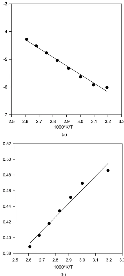
supercritical phase. Whereas, we predict that deviation concern to be inaccurate values of A2. For this purpose we have plotted A versus 1T that intercept shows value ofA2. Figures 1(a) and (b) show plots of A and B versus inverse temperature for C17H36. It is clear that A and B versus inverse temperature are not first order.

2.2. Second Order Temperature Dependency of Parameters

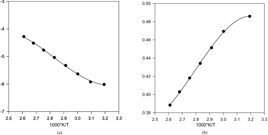
In order to solve this problem, the linear isotherm regular-ity equation of state in the form of truncated temperature series of A and B parameters have been developed to second order for dense fluids. Figures 2(a) and (b) show plots of A and B parameters versus inverse temperature for C17H36 fluid. It is clear that A and B versus inverse tem-perature are second order. Thus, we obtain extended pa-rameters A and B resulted in the second order equation, as

3 2

1 2

A A A A

T T

   (7)

3 2

1 2

B B

T T

  

B B (8)

The starting point in the derivation is Equation (2) again. By substitution of Equations (7) and (8) in Equa-tion (2) we obtain the pressure for dense fluid.

3

3 3 3

5 3

1 2

5 5

1 2

A R A R

T B R

T p RT A RT

B RT B R



 

  

 



 



 1 LIR TPC

(9)

First, second and third temperature coefficients and their temperature derivatives were calculated from this model and the final result is for the thermal pressure co-efficient to form .

3 3 3

2

5 3

2 1

5 1

A R R

T B R

T

p _{R A}

T

B R 



 

 

 _{  }

_ 

 

  



1, 3, 1, 3

(10)

As Equation (10) shows, that it is possible to calculate the thermal pressure coefficient at each density and tem-perature by knowing

2.5 2.6 2.7 2.8 2.9 3.0 3.1 3.2 3.3

1000*K/T

(a)

0.38 0.40 0.42 0.44 0.46 0.48 0.50 0.52

2.5 2.6 2.7 2.8 2.9 3.0 3.1 3.2 3.3

1000*K/T

(b)

Figure 1. (a) Plot of A versus inverse temperature. The solid line is the linear fit to the A data points, for C17H36; (b) Plot

of B versus inverse temperature. The solid line is the linear fit for C17H36.

have plotted extending parameters of A and B versus

1T

1, 3, 1, 3

that intercept and coefficients show the values ofA A B B that are given in Table 2.

2.3. Third Order Temperature Dependency of Parameters

In another step, we test to form of truncated temperature series of A and B parameters to third order (Figures 3(a)

and (b)).

[image:3.595.58.288.111.196.2]

(4)

-7 -6 -5 -4 -3

2.5 2.6 2.7 2.8 2.9 3.0 3.1 3.2 3.3 0.38 0.40 0.42 0.44 0.46 0.48 0.50

2.5 2.6 2.7 2.8 2.9 3.0 3.1 3.2 3.3

1000*K/T 1000*K/T

(a) (b)

Figure 2. (a) Plot of A versus inverse temperature. The solid line is the linear fit to the A data points, for C17H36; (b) Plot of B

versus inverse temperature. The solid line is the linear fit for C17H36 .

-7 -6 -5 -4 -3

2.5 2.6 2.7 2.8 2.9 3.0 3.1 3.2 3.3

0.38 0.40 0.42 0.44 0.46 0.48 0.50

2.5 2.6 2.7 2.8 2.9 3.0 3.1 3.2 3.3

1000*K/T 1000*K/T

(a) (b)

Figure 3. (a) Plot of A versus inverse temperature. The solid line is the linear fit to the A data points, for C17H36; (b) Plot of B

[image:4.595.74.526.86.314.2]

versus inverse temperature. The solid line is the linear fit for C17H36 .

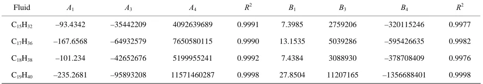
Table 2. The calculated values of A1, A3, using Equation (7) and B1, B3, using Equation (8) for different fluids and the

coeffi-cient of determination (R2).

Fluid A1 A3 R2 B1 B3 R2

C15H32 10.9156 816865.8686 0.9961 –0.7634 –76880.7076 0.9933

C17H36 17.7236 1653515.0792 0.9950 –1.2741 –142952.2089 0.9909

C18H38 24.7654 2604637.9359 0.9965 –1.7380 –207122.0903 0.9933

C19H40 19.3144 1507260.4826 0.9993 –1.9978 –212489.3619 0.9987

[image:4.595.74.527.355.583.2] [image:4.595.56.539.648.735.2]

(5)

3 2 4 2 3 A 1 A A

T T T

A A  (11)

3

2 4

2 3 B

B B

T T T 1

B B  (12)

The starting point in the derivation is Equation (2) again. By substitution of Equations (11) and (12) in Equation (2) we obtain the pressure for dense fluid.

3 3 4 2 5 4 2 A R

3 3 3

1 2

5

5 5 3

1 2 A R T B R T 

p RT A RT A R T B R B RT B R

T                 

 2 LIR TPC

(13)

The final result is for the thermal pressure coefficient to form .

3 3 3 1 5 5 3 1 2 3 4 2 3 5 4 2 3 2

A R A R

T T

B R

T T

p

R A R T B R B R          _{  } _ _        

4, 1, 3, 4

(14)

That based on Equation (14) to obtain the thermal pressure coefficient, it is necessary to determine values

1, 3,

A A A B B B

 0

 1 TPC

 2 TPC that these values are given in Table

3.

3. Experimental Tests and Discussion

Specific experiments on heavy hydrocarbons to set up a base which can then be used to define new models spe-cially adapted to these complex mixtures. With this aim in mind, an investigation was carried out on pure hydro-carbons with more than 16 carbon atoms, as hexadecane is the crucial point beyond which data in the literature become very fragmentary [1,3]. This paper describes the behavior of the thermal pressure coefficients, measured between pressures of 0.1 and 150 MPa and temperatures of 313.15 and 383.15 K, for liquid n-Pentadecane (C15), n-Heptadecane (C17), n-octadecane (C18) and n-nonadecane (C19). When measurements of this property are carried out over a sufficiently wide range of pressures (as is the case in this work), the thermal pressure coefficients data can be integrated so as to generate other thermo-physical properties (including density), provided that an

appropriate set of initial conditions is available [19-23]. These include knowledge of the density and the thermal pressure coefficients data at a reference pressure (the most convenient being atmospheric pressure). As these additional measurements have already been performed, we were able to deduce, by means of numerical integra-tion algorithms which have already been tested on vari-ous occasions [1,3], the behavior up to P = 150 MPa of the following properties: density, thermal pressure, in-ternal pressure and inin-ternal energy.

The thermal pressure coefficient is computed for dense fluids of liquid and super critical using three different models. C17H36 serve as our primary test fluids because of the abundance of available pVT data. When we re-stricted temperature series of A and B parameters to first order it has been seen that the points from the low densi-ties for TPCLIR deviate significantly from the experi-mental data [24,25]. To decrease adequately deviation thermal pressure coefficient from the experimental data, it was necessary to extension temperature series of A and

B parameters to second order [5]. Nevertheless, for some mono atomic fluid similar to Ar that the temperature de-pendencies of the A and B parameters themselves are satisfactory to first order. The present approach to ob-taining the thermal pressure coefficient from pVT data contrasts with the experimental data by extension tem-perature series of A and B parameters to second order and its derivatives. That, the thermal pressure coefficient give to form LIR.

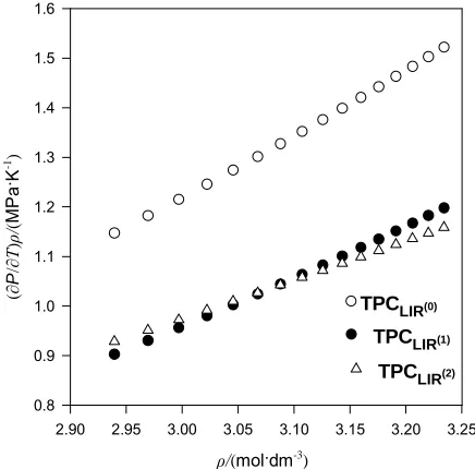
[image:5.595.55.541.652.737.2]

We also considered an even more accurate estimates namely, extension temperature series of A and B pa-rameters to third order. Then we introduce the explicit parameters and temperature dependencies resulting from the pVT data. The final result is for thermal pressure co-efficient to form LIR. In contrast, Figures 4 to 7 show the LIR(0) values ofthethermal pressure coefficient versus density for C15H32, C17H36, C18H38 and C19H40 of liquid that are compared with the thermal pressure coef-ficient using the LIR(1) and LIR(2) at 333.15 and 343.15 K, respectively. Although all three models capture the qua- litative features for dense fluids, only the calculated val-ues of the thermal pressure coefficient using the LIR(1) and LIR(2) model produce quantitative agreement.

Table 3. The calculated values of A1, A3, A4, using Equation (11) and B1, B3, B4 using Equation (12) for different fluids and the

coefficient of determination (R2).

R2 B4 B3 B1 R2 A4 A3 A1 Fluid 0.9977 –320115246 2759206 7.3985 0.9991 4092639689 –35442209 –93.4342

C15H32

0.9982 –595426635 5039286 13.1535 0.9990 7650580115 –64932579 –167.6568

C17H36

0.9976 –378708409 3088930 7.4384 0.9992 5199955241 –42652676 –101.234

C18H38

0.9998 –1356688401 11207165 27.8504 0.9998 11571460287 –95893208 –235.2681

(6)

/ ( mol dm-3 )

2.95 3.00 3.05 3.10 3.15 3.20

0 1 2 3 4 3.25 3.30 (  P /    )  / ( M P a K -1 ) 0.8 0.9 1.0 1.1 1.2 1.3 1.4 1.5 1.6

TPC_LIR(0)

TPC_LIR(1)

TPC_LIR(2)

ρ/(mol·dm-3₎

[image:6.595.312.536.85.306.2]

( ∂ P / ∂ T ) ρ / ( MP a · K -1)

Figure 4. The thermal pressure coefficient values using LIR(0), versus density for C18H38 fluid compared with the

thermal pressure coefficient using LIR(1) and LIR(2) at 333.15 K.

/ (mol dm-3

)

2.90 2.95 3.00 3.05 3.10 3.15 3.20 3.25

(  P /    ) / ( M P a K -1 ) 0.8 0.9 1.0 1.1 1.2 1.3 1.4 1.5 1.6

TPC_LIR(0)

TPC_LIR(1)

TPC_LIR(2)

( ∂ P / ∂ T ) ρ / ( MP a · K -1)

[image:6.595.65.283.85.312.2]

ρ/(mol·dm-3₎

Figure 5. The thermal pressure coefficient values using LIR(0),versus density for C18H38 fluid compared with the

4. Results

In this paper, we derive an expression for as the thermal pressure coefficient of C15H32, C17H36, C18H38 and C19H40 dense fluids using the linear isotherm regularity[1,3,18]. Unlike previous models, it has been shown in this work that, the thermal pressure coefficient can be obtained

/ (mol dm-3

) (  P /    ) / ( M P a K -1 )

2.80 2.85 2.90 2.95 3.00 3.05 3.10

TPC_LIR(0)

TPCLIR(1)

( ∂ P / ∂ T ) ρ / ( MP a · K -1 )

TPCLIR(2)

[image:6.595.313.534.372.588.2]

ρ/(mol·dm-3)

Figure 6. The thermal pressure coefficient values using LIR(0), versus density for C19H40 fluid compared with the

thermal pressure coefficient using LIR(1) and LIR(2) at 333.15 K. 0.8 1.0 1.2 1.4 1.6 1.8 2.0

/ (mol dm-3 )

(  P /   ) / (M P a K -1 )

2.75 2.80 2.85 2.90 2.95 3.00 3.05 3.10

TPC_LIR(0)

TPC_LIR(1)

( ∂ P / ∂ T ) ρ / ( MP a · K -1 )

TPC_LIR(2)

ρ/(mol·dm-3₎

Figure 7. The thermal pressure coefficient values using LIR(0),versus density for C19H40 fluid compared with the

[image:6.595.64.282.378.593.2]

(7)

sure coefficient of dense fluids of the monatomic is doubtful [18]. The validity of the use of the linear iso-therm regularity equation state for calculating the iso-thermal pressure coefficient of dense fluids of the polyatomic is not also precise [5]. In this work, it has been shown that the temperature dependences of the intercept and slope of using linear isotherm regularity are nonlinear. This prob-lem has led us to try to obtain the expression for the ther-mal pressure coefficient using the extending the intercept and slope of the linearity parameters versus inversion of temperature to 2 order. The thermal pressure coefficient are predicted from this simple model are in good agree-ment with experiagree-mental data. The results show the accu-racy of this method is general quite good.

5. Acknowledgements

The authors thank the Payame Noor University for finan- cial support.

REFERENCES

[1] J. L. Daridon, H. Carrier and B. Lagourette, “Pressure Dependence of the Thermophysical Properties of n-Pen- tadecane and n-Heptadecane,” International Journal of

Thermophysics, Vol. 23, No. 3, 2002, pp. 697-708. doi:10.1023/A:1015451020209

[2] L. Boltzmann, “Lectures on Gas Theory,” University of California Press, Berkeley, 1964.

[3] S. Dutour, J. L. Daridon and B. Lagourette, “Pressure and Temperature Dependence of the Speed of Sound and Re-lated Properties in Normal Octadecane and Nonadecane,”

International Journal of Thermophysics, Vol. 21, No. 1, 2000, pp. 173-184. doi:10.1023/A:1006665006643 [4] V. Moeini, “A New Regularity for Internal Pressure of

Dense Fluids,” Journal of Physical Chemistry B, Vol. 110, No. 7, 2006, pp. 3271-3275. doi:10.1021/jp0547764 [5] V. Moeini, F. Ashrafi, M. Karri and H. Rahimi,

“Calcula-tion of Thermal Pressure Coefficient of Dense Fluids Us-ing the Linear Isotherm Regularity,” Journal of Physics Condensed Matter, Vol. 20, No. 7, 2008.

doi:10.1088/0953-8984/20/7/075102

[6] V. Moeini, “Internal Pressures of Lithium and Cesium Fluids at Different Temperatures,” Journal of Chemical &

Engineering Data, Vol. 55, No. 3, 2010, pp.1093-1099. doi:10.1021/je900538q

[7] V. Moeini and M. Deilam, “Determination of Molecular Diameter by pVT,” ISRN Physical Chemistry, Vol. 2012, 2012. doi:10.5402/2012/521827

[8] V. Moeini, “Internal Pressures of Sodium, Potassium, and Rubidium Fluids at Different Temperatures,” Journal of Chemical & Engineering Data, Vol. 55, No. 12, 2010, pp. 5673-5680. doi:10.1021/je100627c

[9] R. B. Stewart and T. Jacobsen, “Thermodynamic Proper-ties of Argon from the Triple Point to 1200 K with Pres-sures to 1000 MPa,” Journal of Physical and Chemical Reference Data, Vol. 18, No. 2, 1989, pp. 639-798.

doi:org/10.1063/1.555829

[10] R. D. Goodwin, “Carbonmonoxide Thermophysical Prop-erties from 68 to 1000 K at Pressures to 100 MPa,”

Jour-nal of Physical and Chemical Reference Data, Vol. 14, No. 4, 1985, pp. 849-933. doi:org/10.1063/1.555742 [11] R. Span and W. Wagner, “A New Equation of State for

Carbon Dioxide Covering the Fluid Region from the Tri-ple-Point Temperature to 1100 K at Pressures up to 800 MPa,” Journal of Physical and Chemical Reference Data, Vol. 25, No. 6, 1996, pp. 1509-1596.

doi:org/10.1063/1.555991

[12] R. T. Jacobsen, R. B. Stewart and M. Jahangiri, “Ther-modynamic Properties of Nitrogen from the Freezing Line to 2000 K at Pressures to 1000 MPa,” Journal of

Physical and Chemical Reference Data, Vol. 15, No. 2, 1986, pp. 735-909. doi:org/10.1063/1.555754

[13] B. A. Younglove and J. F. Ely, “Thermophysical Proper-ties of Fluids. II. Methane, Ethane, Propane, Isobutane, and Normal Butane,” Journal of Physical and Chemical

Reference Data, Vol. 16, No. 4, 1987, pp. 577-799. doi:org/10.1063/1.555785

[14] R. D. Goodwin, “Benzene Thermophysical Properties from 279 to 900 K at Pressures to 1000 Bar,” Journal of

[15] R. D. Goodwin, “Toluene Thermophysical Properties from 178 to 800 K at Pressures to 1000 Bar ,” Journal of

[16] Y. Ghayeb, B. Najafi, V. Moeini and G. Parsafar, “Cal-culation of the Viscosity of Supercritical Fluids Based on the Modified Enskog Theory,” High Temperatures-High Pressures, Vol. 35-36, No. 2, 2003, pp. 217-226. doi:10.1068/htjr056

[17] G. A. Parsafar, V. Moeini and B. Najafi, “Pressure De-pendence of Liquid Vapor Pressure: An Improved Gibbs Prediction,” Iranian Journal of Chemistry and Chemical

Engineering, Vol. 20, No. 1, 2001, pp. 37-43.

[18] G. Parsafar and E. A. Mason, “Linear Isotherms for Dense Fluids: A New Regularity,” Journal of Physical

Chemistry, Vol. 97, No. 35, 1993, pp. 9048-9053. doi:10.1021/j100137a035

[19] G. Parsafar and E. A. Mason, “Linear Isotherms for Dense Fluids: Extension to Mixtures,” Journal of

Physi-cal Chemistry, Vol. 98, No. 7, 1994, pp. 1962-1967. doi:10.1021/j100058a040

[20] G. A. Few and M. Rigby, “Thermal Pressure Coefficient and Internal Pressure of 2,2-Dimethylpropane,” Journal

of Physical Chemistry, Vol. 79, No. 15, 1975, pp. 1543- 1546. doi:10.1021/j100582a013

[21] G. R. Driver and A. G. Williamson, “Thermal Pressure Coefficients of Di-n-alkyl Ethers,” Journal of Chemical

& Engineering Data, Vol. 17, No. 1, 1972, pp. 65-66. doi:10.1021/je60052a034

[22] G. C. Fortune and G. N. Malcolm, “Thermal Pressure Coefficient and the Entropy of Melting at Constant Vol-ume of Isotactic Polypropylene,” Journal of Physical

(8)

doi:10.1021/j100863a015

[23] J. M. Harder, M. Silbert, I. Yokoyama and W. H. Young, “The Thermal Pressure Coefficients and Heat Capacities of Simple Liquid Metals ,” Journal of Physics F: Metal

Physics, Vol. 9, No. 6, 1979. doi:10.1088/0305-4608/9/6/007

[24] T. M. Reed and K. E. Gubbins, “Applied Statistical Me-chanics,” McGraw-Hill, Inc., New York, 1973.