Modelling and forecasting the demand for electric energy in New Zealand

MODELLING AND FORECASTING THE

DEMAND (FOR ELECTRIC ENERGY IN NE\V ZEALAND

A thesis presented for the

degree of Master of Engineering in Electrical Engineering in the University of Canterbury

by

M.J. Turnbull B.E.(Hons)

[""'..

1974

ABSTRACT

This thesis studies the demand for electric energy and ways of forecasting it, as an aid to the economical design and operation of electric power systems. An examination of the nature of

consumers demands leads to a two part model of the demand. Long term growth of demand is shown to be determined by the way

the numbers of appliances ow11ed by consumers increases, while the

sho~t term daily, weekly and seasonal demand fluctuations ~esult

from the way consumers use their appliances. A number of forecasting methods utilizing this model are studied.

The accuracy of a demand forecast influences the amount of

I wish to thank the many people who have helped me, through advice 1 discussion 1 criticism and encouragement, to ~:~omplete

this thesis. Special thanks are due to my supervisor:31

TABLE OF CONTENTS

PAGE

CHAPTER

1

INTRODUCTION

1. 1

A background to the thesis 'l

1.2

Definition of problems examined 7 ..

..J

1.3

Thesis organization and chapter

summary :>

1.4

Data processing and computer programs 9

CHAPTEH

2

THE NATURE OF THE DEMAND

2.1

Introduction

14

2.2

Classification of energy consumers

111-2.3

The demand for electric energy

16

2.4

Growth of energy usage

22

2.5

Summary

26

CHAPTER

3

DESIRABLE MODELLING AND FORECASTING

ACCURACY

3.1 .

Introduction

37

3.2.

The criterion of sufficient accur ;,cy

38

3.3

Reserve capacity for plant outage and

forecast uncertainty

41

3·5

Accuracy of short term demand forecasts

3·6

Accuracy of long term demand forecasts

3-7

Energy usage forecasts

3·8

.Summary

CHAP1'ER

4

THE STATE OF THE ART

4.1

Introduction

4.2

Long term forecasting methods

4.3

Weather

-

load models

4.4

Short term forecasts for system

operation

L~ •

5

Conclusions

CHAPTER

₅

THE LOAD GROWTH PROCESS

5.1

Introduction

5.2

Load growth for a class of consumers

5·3

The growth of domestic energy requirements

5·

~- Growth of non-domestic energy requirements

5·5

Summary

CHAP'J.'ER 6 SHORT TERM LOAD BEHAVIOUR

6.1

Introduction

6.2

Modelling the seasonal behaviour of the

load

6.3

Determination of the components of the

daily load curve

48

54

56

60

67

68

82

91

96

104

106

108

120

132

139

141

6.4

Climate and short term load behaviour

155

6.5

Forecasting a~plications

164

6.6

Conclusions

168

CHAP'I'ER 7 CONCLUSIONS AND RECOMMENDATIONS

7.1 Conclusions

7.2

Recommendations

APPENDIX A DETERMINATION OF EXPECTED DEFICIENCY

OF DEMAND

APPENDIX B A DERIVATION OF MEAN SQUARE ERROR OF THE KARHUNEN LOEVE EXPANSION

APPENDIX C

APPENDIX D

REFERENCES

RESULTS OF EXPERIHENTAL' FORECASTS MADE USING FARMER'S METHOD

DEMAND ... TEMPERA1.'URE SCAT'rER DIAGRAI1S

FOR AN URBAN LOAD

'1 )1

•197

200

210

LIST OF FIGURES

PAGE

FIGUBE 1 • •J The place of a load model in system

operation and planning 11

1. 2 Influence of environment on the demand

{or electric Energy 12

1. 3 Thesis structure 13

2.1 Number of domestic and non-domestic

consumers and their ratio:: New Zealand 28 2.2(a)Daily load curves for each day of the

week: Christchurch MED 29

2.2(b)Mean weekday load curv~s: Christchurch

MED 30

2.3(a)Monthly average daily load curves for

Christchurch MED 31

2.3(b)Monthl~.r average daily load curves fo:t•

Woolst<:•n Nos. 1 & 2 feeders 32

2~3(c)MonthJy average daily load curves for

Riccarton BC 33

2.4 Share of NZ energy market met by major

energy sources 34

NZ annual energy usage and max. demand

₃₅

2.7 Average ~nergy usage by domestic and

3.1 Cast of unc:ertainty

3.2 Costs of uncertainty and plant o_utage

reserve

3.3 Simple

18

generator and single load

power system

3.4 Risk of not meeting forecast demands

3.5 Seasonal energy balance

3.6 Probability that energy required

exceeds that available

4.1 Typical forecasting strategy:

weather-load model

4.2 Error histogram for scaling methoa

Growth of domestic consumer numbers

5.2(a)Age group at death

5.2(b)Age group at marriage

5.3 Growth of domestic consumer numbeEs:

c.f. 11_{birth and death}11 _{model and actual}

occurrences

5.4 Non-domestic consumer numbers as a

function of population

Non-domestic energy usage and GNP

6.1 Christchurch MED: seasonal changes in

daily energy usage

6.2 Initial component load curves

62

62

63

64

65

·66

102

103

136

137

138

170

6.3 Shape of evening component with ' j '

Load curves for Tuesdays of one year

6.5 Statistical summary of normalized daily

load curves

6.6 Final component load curves and scale

factors

6.7 Mis-match between 3-component model and

raw data

6.8 Load curves generated by 3-component

model

6.9 Eigenvectors and spectral coefficients

171

172

173

173

174

175

for 11_Tuesday11 _{load curves 176}

6.10 Operation of Karhunen Loeve expansion 177

6.11 Fourier series approximation 178

6.12

6.13

6.14

Fourier components for'one year's demands179

Load curves generated by "Fourier" model 180

Demand and temperature on 3.10.67 181

6.15 Demand and lagged temp. at interval 40 182

6.16 Estimated coefficients for demand-lagged

temp. model

6.17 Residual demand for three demand-climate

models

6.18 Estimated coefficients for

demand-temp-daylight model

6.19 Load curves generated by demand-weather

model

6.20 Deviation of North Is. wdighted temps.

from mean

'182

LIST OF TABLES

TABLE PAGE

2& 1 Annual sales of consumer appliances. 27

3.1 Generator parameters. 63

4.

'1 Commonly used trend curves.

₉₉

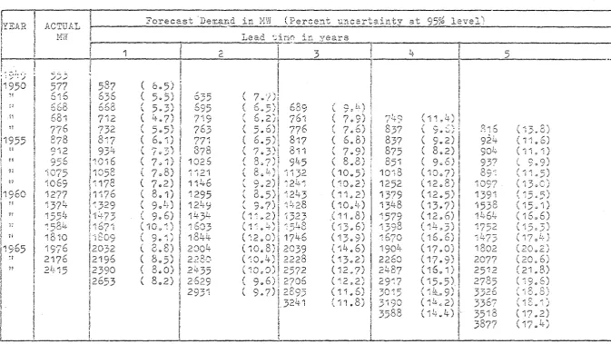
4.2 Annual maximum demand forecasts (

N.z.

) 100

1

IN'l'RODUC'l'ION

A comprehensive model of the load on the New Zealand electric p(~er system is the long term goal of the work presented in this

t.::1esis. This fuodel is to be used for forecasting consumer demands for electric energy.

Electric energy cannot be stored economically in the. amounts

typical of a power sy~tem and must be generated as required. To maintain the quality of the energy supply (i~e. voltage and frequency) at predetermined levels the power output of the generating system must remain equal to the demand for energy. Output cannot respond instantaneously to changes in demand due to restrictions imposed by

plant parameters

(3, 4, 5)

or9 in the worst case, because the total

generating capacity of the system is exceeded. Demand forecasts

enable the initiation of adjustments to the system's power output before any changes in the demand occur. The lead time of the

forec~2t should equal, or exceed~ the time required for the particular adju::;tment~

System operation requires demand forecasts over lead times

frbm a few minutes to a few days for

(a) the adjustment of the output of plant already operatingg and

(b) scheduling the start up of additional generators.

installation of additional planto Thus future system operators must operate the system to meet the actual deman~s from the amount of generating capacity installed on the basis of these long term forecasts.

2

The management of a powe1· system may elect to meet all demands for electric energy from consumers or, alternatively, devise controls to restrict the demand to soffie desirable value. For example,

supply authorities in New Zealand control electric water heating with the aim of reducing costs to the consumero The procedure for designing appropriate 0ontrols is equivalent to forecasting the unconstrained demand ~nd then determining the adjustments required

(6).

In this nituation a model of the load is required which is able to confirm that a proposed control action will have

the desired effect.

Several methods of forecasting demand and energy requirements

over all lead times h?ve been described in the literature. A comprehensive and cri~ical review of these methods is contained in chapter 4 of this ~hesis; shoyter reviews are given by Statiton and Gupta {1) and Ma~thewman and Nicholson (2)~ All methods require a model of the. load Jnd its beha~iour; this may be a time series

representation of hitJtorical dema.nds or a more complex representation of the structure (ol' rules of behaviour) of the load. The best forecasts, in a min:..rnum error mmse₉ can only be obtained if the

model is appropriatJ to the particular load (109 11).

The New Zealan·l power system is c6mposed of a central (state-run)

The central organization generates and sellF electric energy in bulk to the supply authorities which·in tu~n ~istribute it to

individual consumers. At present supply authorities estimate

3

their annual maximum demands and energy requirements in isolation. These separate forecasts are then combined to form national forecasts

which are then used in planning future plant requirements (71 8, 9)~

In this way specialist local knowledge is introduced into the national forecasts; without it there are limits on the detail in

the ~ational forecasts

(11, 17).

The literature contains no

evidence of any study of the New Ze~land load to ensure the models

in use are appropriate. Such a study forms a considerable part

of the work presented here. This thesis brings together~ for the first time in New Zealand9 a comprehensive review o~ available

forecasting methods and a comprehensive ctudy of t~e New Zealand load.,

1 .. 2 Definition of Problems Examined in the Thes~.s

An "overviewfl of the place of a comprehensive load model in power system planning and operation is provided in Figure 1~1. The actual demand for electric energy results f:r:om the action !Jf

the environment in which the power system exist''' on the conGumerso In general there is a time lag between the occt:. ·~renee of a11 "event 11

in the environment and a change in the demand

:.n

response to that

"event"; this time lag varies between enviromc:ent variables. If a known ehvironment is applied to an appropriate model of the load then the demand can be forecast over lead time: at least equal to

used.

4

The application of an actual or projected environment to the load model, resulting in a forecast value of demand0 is shown in parallel with the real world .in Figure 1.1. Information on actual

and forecast demands is supplied to the generation planning and

decision processes. These processes determine the amount of

g :merat:i.on capacity (including reserve) required to ensure the forecast demand .will be met with the desired degree of confidence (usually of the order of

99e99% (16));

the allocation of reserve

capacity is discussed in greater depth in Chapter

3.

Two particular aspects of figure 1.1 are examined in this thesis;

(a) the modelling of the load and its response to the environment, and

(b) the accuracy with which it is necessary to forecast the dem,:mdG

The way in which the environment determines the demand is

shown in greater detail in Figure 1.2. Not all environment variables have the same effect on the load; in Figure 1.2 these variables form two distinct groups;

(11) those which govern the number of appliances which

consumers have available for connecting to the

distribution network (i.eo the potential demand)~ and (b) those which determine the way consumers use the appliances

which they own.

For th~ majority of appliance types only a few discrete rates of energy usage are possible. These are fixed when the appliance is

In an ideal case? a knowledge of the number of appliances9

their types9 and the way they are used would be sufficient to

5

The problemH of long and short term forecasting are illustrated by Figure 1.2. Short term forecasting (lead times up to a few days)

is essentially concerned with how consumers use their appliances as~ over the usual lead times, the appliance numbers are known and

ro~atively constant. Provided the way appliances are used remains ~ubstantially constant over periods of several years the long term

forecasting problem is essentially the determination of growth in

appliance numbers.

To summarize, the principal problems examined in this thesis are (a) the modelling of load growth as represented by the growth

of appliance numbers;

(b) the modelling of the way these appliances are used by

consumers,. and

(c) the accuracy with which it is desirable to forecast the demand (and hence how well the models must repres~nt the real system)$

1. 3 Th~sis Organiz,atioD: ... E.!ld Ch_Epter Summa.!:ll. .

Each chapter of the thesis is as self-contained as possible,

consiatent with a satisfactory treatment of the problems.

chapters build on earlier work with a minimum of references in

earli~r chapters to later oneso

thesis is shown in Figure 1.3.

The basic structure of the

There are two parallel lines of

devHlopment. In Ohapter 2 the overall load modelling problem is

formulated; this leads directly to the discussions of load growth in Chapter 5 and of the demand (or way appliances are used) in

6

of the state of tha art (i.e. load modellin and demand forecasting) in Chapter 4o The approaches adopted in Chapters

5

and

6

are

influenced by this review. Chapter

7

summarizes the principal

achievements of the thesis and makes recommendations for further worka Appendices are used for clerivationsg experimental result;; and a

certain amount of data which is presented as a sequence (,f diagrams&

References are listed together at the end of the thesis, in order of appearanceo

Detailed formulation of the modelling problem is the subject

of Chapter 2. This formulation, following the outline in Figure 1.2₁ treats the problem in two parts. The first par·c is modelling

the process governing appliance number growtho ModNlling the

usage of appl~ances forms the second part.

In Chapter

5

the load growth process is further divided into

two parts:

(a) that which determines consumer numbers₉ and (b) that which determines the number of app~iances a

consumer owns.

The nature of these processes varies between conlumer types.

A type of birth and death process is advanced to explain domestic

consumer numberso Using this model consumer nPnbers can b11 forecast for lead times up to about 15 years from known information. This is superior to models which require the prior extr<lpolation o:f

11_indepex~dent11 _{variables, for example the "housi·,;g sta.rts" index in thA}

correlation model used by Godard (12). Electrl.cal appliances are

7

consumer durableso The work of Pyatt (13) ~n models· of the

accumulation of durables by households is used to develop a model,

of the growth of a dome~tic consumer's ownership of applianceaG Non=domestic consumer numbers cannot be modelled by a simple birth and death process as in the domestic case. Neith::r are there any useful (for forecasting) rules governing the number )f appliances

owned by individual consumerso

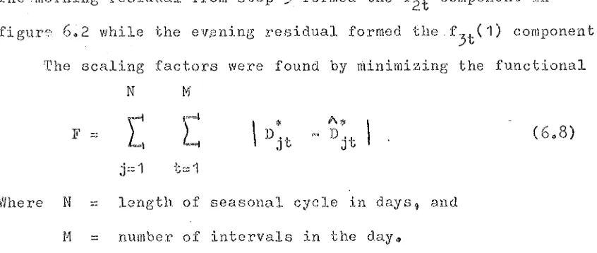
Models of appliance usage, which are the subject of Chapter

6

9 have been based on day to day changes in the daily loa~ curves. These changes reflect day to day vatiations in the way appliances

are usedo The shape of the daily load curve itself is determined by the aggregation of these usage patterns over the day. While the model development actually proceeded in an i ter:.ttive fashion the chief results only are presented;' a complete J'ecorcl would occupy too much space and serve no useful purpose~

In the approach adopted here each da;y of th<: week is modelled separately, thus avoiding the need for the da.y-ol-week factors etc. used, for example~ by Davies (14); this approac~ is equivalAnt to the weekly load curve approach used recently by Christiaans~ (10).

In the results and discussion attention is conf~ned _. to one par~icular _.

day of the week - Tuesd~y~

The discussion starts with a model of the observed seasonal changes in daily load curve shapeo Three daiJ.y load components~ the shapes of which are obtained artificially₁ are shown to be

sufficient to explain the mean seasonal behavi0ur. Witl1 this model

it is pdssible to generate a sequence of dail~ load curves for a

8

seasonal movements ate assumed basically r nusoidal in naturea

A Fourier series representation of the mean seasonal behaviour is also discussed. It is shown that an adequate representation of the mean behaviour is bbtained using only a

constant term and the first sine term to represent the integrated

demand in each daily interval. The Karhunen-Loeve expansion

(2,15)

is also investigated as a model of seasonal behaviour; it turns out that it is not suitable for this purpose although it has been used in very short term forecasting applications (2).

In a third model demand is related to the inte~nal temperature

of buildings and to hours of daylight. A complex non-linear

relationship between demand and internal temperat11re was first used by Davies (14) to model the demand at the time of the daily maxima.

In Chapter

6

a piece-wise linear relationship ie applied to all intervals of the day. The presence, or absenc~, of daylight at each daily interval (which is a function of th<! time of the year) determines whether a constant block of load~ attributable to lighting9

is present or note

A considerable amount of variation in th~ demand is not

explained by this model~ Neither can it be 11xplained satisfactorily

by introducing further weather parameters. It is concluded that

this variation arises from vagaries of human behaviour and that it cannot be reduced without extremely compreheJtsive (and expensive)

load control measures. This residual vari~~ion sets nn upper limit

on the achievable demand forecasting accuracy. Considerable

9

In Chapter 3 a cri~eriori is derived for determining tho accuracy with which it is desirable tci forecast the demand; The

desirable accuracy minimizes the total cost of allowing for

uncertainty in the forecast and of making the forecast. Using this criterion it is shown that th:~re is no advantage in reducing the uncertainty in demand (and en9rgy) forecasts below an amount set by plant unreliabilityo

'l'his criterion also means that forecasting methods must be

compared on the basis of tho uncertainty in the forecasts at some

stated confidence level; the amount of spare capacity required to

ensure the supply achieven the reliability specified by management is directly related to this uncertainty. The commonly used measure of comparison between methods is the achieved forecasting error (i.eo

·,

the difference between forecast value and actual value)

(1

9

11, 17);

this· may lead to mis:ple.ced optimism as to the forecasi;ing accuracy of a method and to ins\!.ffici.ent reserve capacity being provided for a given reliability r1.'quirement.

A comprehensive ceview of exL;;ting electric energy forecasting

methods constitutes C1_1a:i?ter

_4.

_{Methods are .compared bsing the}

uncertainty measure ~arived in Ctapter

3Q

The methodology of demand and energy forecastL:,g over all lead times is ex<.'.mined critic ally ..

The considerabJ~ amount of data processing required during this project was carried out with the aid of the computer at the University

10

trend extrapolation model, the scaling metho and the Karhunen-Loeve expansion method in Chapter

4

and.the regression analysis in Chapt~r

6.

For simplicity these programs employed standard sub-routines,

where these were available9 to carry out the required computations, e.g. statistical analysis~ regression analysis, eigen val1w evaluation

and various matrix operations such as inversion. Most programming

effort was devoted to organizing data for input to these sub-routines-and to displaying the results of the computations on the l~ne printer and on an incremental drum plotter. No new computational techniques were developed as such.

The majority of the data used and some programs relating to its

input to the computer are described in a Departmental Memorandum, see Several other sub-routines*,for displayin~ data on the line printer or drum plotter9 and assembly language versions (for increased speed) of standard routines are availabl~ in the Electrical

Engineering Department Program Library. A number of illustrations

in this thesis (eGg. Figure 2~2) were prepared us1ng one of these Fortran routines which plots a surface a.s sequence of crons· .. sections 0 :i.n, the

The specific nature of the remaindeJ• of the progJ.'a~s meant that they would be of no benefit to others, Sufficiunt

information is given in the text to enable a rea:;onably com;;>~:~tent person to program any of the computations descrjtedQ

11

~;~:;;+_

.

_I

I

~;:u:~d-~J

.

I

Ftgure

1.1

I

~

__ r

.~·~-.-·!

Gener·ofton

?lanntn(j'

and

Opera'hon

al

DeCISions

The

f/ace

o.P a

M~)de/

oP

}he

ioc1c

1n

syster"tl

op,eratJcH')

and

1)ay

of week and

hol1da~s.

ClrMote •

·DeMand

(rate of

energ

~

tASO

ge )

L1v1ng

Stondnrds.

Level of

.i

'

T

n

cl

us

t

r

1

a

lr

:t.

a

l

J

on.

----r--··--·--1

12

Frgu~"e

1.2

Influence of the

env'ronr"·H~n·r

on

'2

1

Fo

n"t\U

loh on

of (

Lood

Modell1n9

J

"Probler'l

1

5

Load

Growth

~:..._

_ _ _

_

'Process

1

6

J

3

Forecost1nq

Accuraclj

4

State of

+he f.l

rt

CHAPTER 2

THE NATURE OF THE DEHAND

2.1 Introduction

An electric power system supplies electric energy to consumers

distributed throughout a geoaraphical region which may be a city, borough or countye 'l1_{his ch:tpter discusses the consumers and their}

uses for electric energy. The essential features of their demands for electric energy are detarmined. These features form the basis

for the models of the short and long term time behaviour of the demand which are developed in later chapterse The discussion is illustra-ted by the historical beh~viour of the demand in New Zealand.

2.2 Classification of Eiectric Energy Consumers

On the basis of th0ir primary use for electric energy the consumers within the rngion may be grouped into four general

classeso These classes are:

(1) Domestic co~sumers

A domestic ~onsumer is a group of people, e.g. a family₉ living tog·: ther in the same dwelling; c" f $ the household

of econorni1: theory ( 13₁ 19, 20). (2) Industria]. consumers

An indust·.: ial consumer- is an establishment ₁ e. g. a factory~ ''lhich manufactures, mines or processes a

particule? good or range of goods for consumption within,

or export from~ the region$ Energy~ from one or more sources, forms an input to the manufacturing process₉ together Nith labour and raw materials and is used for

requireme~ts of each.consumer are related to the amount of output9 by some .function of the particular process ..

(3)

Commercial consumers

A commercial consumer is an establishment trading in

merchandise or professional services etc. Such

estab-lishments include shops₉ offices, warehouses etc.

Energy is used for heating, lighting and other services

related to the premises, e.g. escalators. Energy is

not, in general, essential to the operations of these consumers but is used for staff and customer convenience,.

(4)

Public services

These consumers provide services to the public such as

street lighting₉ transport (but not including fossil fuelled vehicles) 9 sewage d~sposal etcQ These a:rn, in New Zealand, considered socially necessary and are

commonly operated by. bodies such as city councils.

Energy requirements are related to the number of people served; eego utreet lighting requirements are a function of urban road length which is in turn some function of the number of urban households~

These classes may be further subdivided in particular cases9 e.g. Jelinek (21) has subdivided class 1 on the basis of income and whether the dwelling is a flat or house etco

The number of consumers in each class increases with time

(as some function of the increase in population) and the ratio of

consumer numbers between classes also changes with time. This

is illustrated in figure 2.1 for domestic and non-domestic consumer numbers in New Zealanda

16

2. 3 The dem.'e.nd for electric ene:cg~

2.3o1 Some Terminology

Consu~ers in all classes reque~t a supply of electric energy

by connecting appliances to the supply network. These connected

appliances form the LOAD on the power system. The DEMAND for

electric ene;egy is the rate at which the load uses elect::·ic energy; it is usually measured in units of power, i.e. kilowatts (kW)a

I

Demand may be referred to as "

(a) instantaneous demand which is the rate qf ene~gy

usage at an instant in time, or

(b) integrated demand which is the average rate of energy usage over a time interval of arb1trary length; usually one quarter, one half cr one hour$

(22, 23) ..

The two terms are related by

where

D.

l. :;:::

1;'

~

JTi+t"

~.o D ( t) dt

T. L

:;::: length of interval in hours

D(t) :::: instantaneous demand at time

D. ::; integrated demand over the

1.

t1 and

i th intervt:tl&

The total a_mount of energy used by the load ove:.· a period ((J9T)

hours is9 using instantaneous demand

w

1

T D(t) dt

0

or using integrated demands n

L'

t

D. i::-:1 J.

w ;;:;

(2.1)

( 2. 2)

where n - an integer -~ 1 denoting th~· number of intervals

17

2.3~2 The variation o£ dem~nd with ti~e

Each connected appliance cont~ibutes to .the demand~ The

total demand within the region at a particular ti~e is the sum of the demands of all the appliances connected at that time. Define

A to be the set of all appliances owned by consumers and able to

be connected at any timeq Not all appliances are necessarily connected at time t ; let «t denote a set made up of members of A which are actually connected at .time t : c<t C/1.. If j denotes a·member of A the total i~stantaneous demand at timet may be

written as

D (t)

₌

~

c. (t) _{( 2} ~ l~)

J

j €. ()1, t

where c . ( t) ₌ demnncl. of member j at time t.

J

The magnitude or the demand v~ries in a cyclic manner with

time of day. The de~and at aparticular time of the day also varies with the day r•f week and time of year (29 24). In figure 2.2 the s~ape of th! daily load cycle for different days of the week and for consect·;ive weekday average load curves through tho

year for an urban S1tpply autho:d .. ·cy are shown.,

2.3G3 The number a~d type of the connected appliances Any member 0f the set A may, with a few exceptions, be connec·~ed or di1;connected a.t any time. /1. aingle appliance can be either 1_on9

1 i.e~ connected, or

1_off1

, i.e. disconnected,

at an instant in time (229 25). Let M denote the number of

different types of appliances in A1 ~nd m₁,i

=

1, •• , M~ the

18

appliances of each type; this meand that whether an appliance

is used or not is a function of the Rppliance type but not of

the consumer owning ito The probability that a type i appliance

is 1_{on; at timet is p.(t); the corresponding} 9_off1 _probability

l.

is q.(t).

~ Provided. that tho probability of observing an on-off

or off-on transition is neglLgible then

p.(t) + q.(t) "'1

~ ~

The probability that there will be exactly n. appliances

1

of type i in

expansion of

(p.(t)

~

p ( f)(.t

the set tXt is given by the n.th term

6f

the

1

+

.. m. q. ( t )) J.

1

contains n. type i appliances)

=

l.

( p. ( t ))n~.

1

(2.6)

The mean and variance of the distribution of possible numbers of

type i appliances on at time t is given by

-n. J.

var ( n.) J..

::::

;:::

m.p. (t)

J.. 1

(2.7)

The contribution of type i appliances to the total demand

is obtained by weig:Cting the number of connected appliances

(equations

2.7)

by lhe demand of this type of applianceQ For

single element app] ::.ancE1S, e. gG lights, refrig•:;rators 9 irons~

this is merely the 1ameplate rating~ For multiple element

BP,pliances, e~ge eJ ~ctric ranges~ radiators 91

Gc. ~ it is necessary

to know which elemE.1ts are connected at the time9 and this is

19

elements an:J nelected by the ,c.onmuner the demand :r·emains constant

Soma industrial loads, e.g. motors, are exceptions

as their demand varies in time as a function of the load on the

motor. However for these and multiple element appliances the

expected demand when connected may be used (25). The mean and

nu·ience of the demand from type i appliances becomes

D. (t) --

m·.c.p.

(t)

~ ~ ~ ~

var (D.(t))

=

m.;~

p.(t) q.(t)

1 ~ l 1 1

-?!here c.

).

i

- expected demand of type i . appliance,

·- 1 , • • • , M

Tho total demand from all types of appliance at time t

is

D( t)

=

H

"D.

(t).

Lt 1.

i=1

(2.0)

(2.9)

The form of the distribution cif D(~) is obtained by combining the

M

distributions of equation

2.8.

Provided the demands D.(t) are

1.

independent and M in sufficiently large the central limit theorem

may be applied (259 26). The distribution of D(t) is then

appro::.imately normal with mean and vnriance given by

H

D(t)

--

r:

m.c.p.

-

(t) (2e10)

i=''j l l. :L

l~ _-2

q. ( t)

·•1ar (D(t)) ::

"'

m.c. p. ( t)

''"I 1. ). . J. ).

20

If the set A does not change with t.~e, i.e. M and m.

1

remain constant - which means no growth in ~ppljance numbers, and if the c. , i

=

1,&~ ₁M? do not change botween consecutive

l

periods of use then the only way for the demand to vary is for the p.(t) to vary with time$

l . .

Hence the time sequence of p

1(t) has the same sh~pe as the time pattern of use of appliances of type i Th1J shape

of the load curve is formed from the combination of thruse appliance usage curveso

2.3.4

The determinants of appliance usage patterns

The surroundings and circumstances in which a consumer

exists~ i.e. the environment1 determine the way in ~hich a consumer uses its appliances. The social, econom5.c and climatic aspects of the enviro~ment appe~r to have the most influence.,.

The social environment governs the living and working habits of the regional population~ It dete~min1s₉ for example,

the times of the day when people eat their mealf J watch television

programmes and go to bed

(21, 24

9

27).

It als·: dictates t'h.:1t the majority of industrial and commercial consu~ers do not operate during weekends; thus the on-probabili·~ies of these

consumers' appliances is a function of the day of the week0 The social environment dictates that the probabili~y of an appliance

being on is a function of the time of the day.

The economic environment affects the 1e1·e1 of the demand

21

inc~ease in the amount of production

(28).

Ini ba1ly this

increased production is obt~in~d by working plan~ for longer

hours, thus extending the time for which the on-probability for

industrial appliances is high. Thus this aspect of the

e~vironment modifies the basic time-pattern of use determined

by the social environment. There is no evidence that domestic

Dppliance use is affected by the economic environment although

it affects the number of appliances a consumer owns

(13, 28,

29).

The climatic environment directly affects consumers~

heating and lighting requirements

(14,

30)~ 'l'he seasonal

decreases in me~n air temperaturei for example₉ increase the

probability that heating devices will be in use. Similarly

the increase in hours of darkness increaf3es the period of time

for which lighting is in use1 thus madifying the ·time-pattern

d use of lighting appliances~

The social environment· dictates that the probability of an

appliance being on is a function of the time of the day; the other

aspects of the environment modify the basic time pattornsj Let

denot~ the set of enviroriment variables relevant to the use of

type i appliances. The influence of the environment on D(t)

may be incorporated into equation 2.10 by treating t as the time

of day and modifying p,,(t); _{- .L .} i.e ..

p (type i appliance is on) :::: g. (e. -~

). l

'

t) (2.11)

The mean and variance of the distribution of D(t) then become

H

(t)

l~

""

t)

D

₌

m.c.g. (e.

'

l ~ l l

M (2.12)

var ( D( t))

₌

t

-2 tv ' ...,

m.c.g.(e. ,t)(1-g.(e. ,t))

i::::1 l l l l l l

.,.,

The extent to which any single environment variable

affects the shape of the daily load c,urvo is determined by the

number of appliances it can affect~ In particul~r, where a

load has a large industrial or public service segment the

influence of the climate is Greatly reducedo This effect is

illustrated in figure 2.3 which shows monthly average daily

load curves (weekdays only) against time of year for three NZED

loads, The first was main1.y domestic with no large industrial

consumers, the third was mainly domestic but with one large

industry and the second inuluded railway traction and a large

public lighting.load (a road tunnel)o

2o4 §'rowth in En~~~!~(~

2.4e1 The demand for etergy from all sources

22

To the consumer£. electricity is merely a source of energy,

tho~gh with some uniquJ features such as ease of control and

clean-liness in use. Alt,:rnative sources which a consumer may choose

for a particular appJ ·,cation include coal, oil and gas. The

factors which a cons11.ner considerr~ when mal{ing the choice may be

summarized as (13, 2:., 31, 32):

(a) relative cost of the alternatives,

(b) availab~lity and ease of use of alternatives, (c) .relativ~ efficienciesg and

(d) consume,. tastes and preferences (which may be

influeaced by advertising and social pressures

This list is not exhaustive and the weighting given each factor

varies between diffel.'ent consumers • . As. a consequence of. this

competition between energy sources electricity supplies only a

portion of the regional energy requirementso

The percentages of Ne~ Zealand9_{s total energy}

require-ments met by coal, gas, elecl;ricity and o:i.l for the :,rears 1950~

1967 are shown ~n figure 2~~. In some applications there is

only one commercially feasitlc source, e.g. oil for motor

vehicles. Thus the considerable increase in motor vehi~le

numbers in this period has contributed disproportionately to

the oil share; in 1967 muter vehicles used nearly half of the

oil (29).,

2. L~ <•2 H:i.storice.l growth of electric energy usage

The am0unt of electric energy'used annually in New

Zealand is increasing :tpproximately exponentially at a rate

This figure

alGa shows the ~nnua] half hourly maximum demand is growing in a

similar way at a sim·.lar rateo

23

In the period co~ered by figure

2.5

the population has

also grown but at a Lower rate; approximately

2%

per annum

(33).

An increase in the number of households (domestic consumers) has

accompanied the -popitlation inc;ceaseo This is shown in figure

2o1o The average Jtumber of people per household has decreased

in this time reflol~ing tendencies for young people to leave

home at an earlier 1ge and for young married couples to torm

This increase in popul~tion has increased the demand for consum~r goods and services~ 'Together with a steady increase

in the level of industrial activity this has meant an increase in non-domestic consuwer numbers, see figure 2.1. The rl3. te of

i :tcrease of these consumer numbers has been greater than that

of domestic consumer numbers as a result of increased emphasis un an industrial base for the national economy

(29

9

33)o

These increases in consumer numbers cannot alone explain the observed increases in annual energy usage. This means that the average energy usage per consumer has also increased in this

period9 as show~ in figure 2~7· Three hypotheses can be advanced to explain the increases in average energy usag~:

(a) the annual energy usage of newly formed consumers exceeds that of consumer~ already in existance₁ which remains constant~ This appears to apply

particularly to factories etc where it is difficult to increase anergy usage without extensive changes

to plant and working hours

(29);

(b) there is an increase in consumers' usage of existing

appliances~ This occurs if more overtime, for example, is worked. In the domestic sector there

24

is increasing reliance on electricity rather than coal fires for heating the home; e.g. in the

1961

census

9o9~& of households claimed 11_{mainly electric heating"}

and this figure increased to 38~6% in the

1966

census

(33).

This means that existing electric radiators

(c) 'rhcre is an increase in the number of appliances owned nnd used by consumers. In Table 2.1 the numbers of various domestic appliances sold during

the years 1958-1967 are shown. This data shows a marked increase in the number of electric radiators

sold about the ye~rs 1961-1962. Huch of this increase refleeLs the increased reliance on

electricity for home heating observed in the census figures. Fur~hermore there has been an increase in

25

the percentagm of households with all electric cooking

as the follo•,, ine; census figures show ( 3L~):

1956 - 56.9?:;; 1961 ~ 68.,8?6; 1966 -?8.6%

Annual sale:3 of all the appliances in Table 2~ 1 are ~~ughly tw~ce the increase in domestic consumer numbers which suguests many sales are for replacement purposes and D or₉ :nany households own several appliances of om)

t.y pe •

The above dic:r:u~;sion indicates that all thrt::e hypotheses are true, at least in pE.rt. Unfort',ma.tely there is a lack of data to confirm them sat·.sfactorily I. 29). It is clear, however, that

two processes contr~bute to the growth in annual energy usage: (a) the inc~ease in population and level of

industrLal activity and

(b) the :i.nc:rease in the average energ-;r uaage of

consum<:rs~ which arises from the :3.ccl1mulation of

26

2.5 Summ~

The demand of the system load has been shown to be the sum of the demands of all the connected appliances. Of the set A

of all appliances owned by consumers only a subset «t is connected

r1t any time te The variation of demand with time reflects changes i.n both the set A and the subset o«. t " ·

For short periods of time~ e.g. one or two months~ the set A may be assumed constant. The shape of the daily load c~rve is

then determined by the daily time sequence of probabilities that

different types of appliances are connected. These probabilities

are functions of the time of day and the environment in which the consumer exists"

Over longer periods oftime₉ e.g. six months to several years~

consumers purchase additional appliances. Increases in the

re~ional population and the demand for goods and services within

the region result in increases in the number of consumers, both

domestic and non-domestic. Both these factors increase the

numbe·t• and type of membars of the set A • Consequently, the level of demand at corresponding times in consecutive years

incr<:~ases as does the amount of energy used annually9

A comprehensive model of the demand for electric energy thus haE; two parts. Tho first models the process which chooses the

subt3et Ol.t of the set of all a.ppliances and hence the short term variation of demand~ The second models the process which increases the number and type of appliances which consumers own and hence the

growth of demand and energy usageo

27

Annual sales of consumer appliances (OOO!s)

Type

__

, Yc1.1.r

1958

l-_;>

9

1

_{60 '6·1}

1

_{62 '63}

1

₆₄

_'65

'66 '67 '68

Electric ranges

29

35 33 38 42 38 40

L~4

_{50 52 47}

Refrigerators

63

51

50 56

4L~

_{38 54 53 61 73 73}

Radiators

₃₅

51 1}7

89 155 "136 152 218 222 213 220

Washing machines 3?

36 38 48

L~o

_{40 42 46 47}

₅₁ Lj.lt

Toasters

29

3L~

_{32 52}

61~ L~L~

_{62 83 67 64 75}

Irons (,'

20 35 59 53

_I}

3 78 82 67 63 67

]of'l1estlc 800

--

Q) 0 0 600 0 .

,..__:..-

...

---

...

-- e--- 0 - -

-' .

0- - - · - - - -

~--<>---·---~~---

~---~---

-~---G--

· ·

-. - - - e ·

-- -- -- -- -- -- -- -&...

--e---0--

-.e---G:>

'Ratio

1

1

!

0

-1-Q

7 p::

0

6 ~

' - ' til t... Q) ...0 E ~

:z.

t... Q) 400

E ..

::S

2QOc-(J)

1J)

E

5 .. 0

""0

I

-...

4 0

z

3 .\" 1.)

'

-+-1 [fJ

c

("\

v

Non

-dorr~est1c

l

2

~

r-~--

:-

.---~---

...

--~- ~---~----~-·-·-·

i;

~

-~ l i I I I l 1 1 l ~

N50

F1gur> e

2.

i

lq55' ·1q6o lq65

Nurr1b~" of ·DoMestsc and i\lon-dorr~est1c ConsuMers and

+ha1r

R·::lho:

New .Zealand

f\)

0

ISO

d a lj

or.

wee 1<.

0600 1200

29

·I~ ~

::1.400

Ft

~ u r e

:J..

:J. (a; ) D o. d

'1

I o a. d C.l : r u e s ~ o r e. a.

c.h ·

do.

lj

k of year'

1.-/ee

I d curves

b) Mean weekday ~a£0.

F'•gure 2.2 ( Chl'lstchwrch for year fro'l ' 3 67

n.

t

°

3/.3.68 ·•

31

A 100

150

100

\ )

c 0

E

Q)

0

50

T1r1e of

year.

L I I I I I. I I l__t_L . I I I I I I

._L..._,j__JC----0600 1200 H?OO

/2400

TIMe ·jf do

y

(he>Lirs)

F'1gure

2.3(a) Monlhly

average

dally load curves; Chr1stchurch

.LI --'-' ----'--' _ ! _ _ I I , . . I I I

060 0 1200 1800

T1Me

cf

day (hours)

32

"U

c

0

[

3.2

~

1.6

Tll"1e

of

year

F1qure

2. 3 (b) f"1ontnly averOIJt~

dally

load

(.:urve s

for

0600

1200

1800

T1Me of

day

(hours)

I.

I I

j: .. '_

--~

24"00

/

1="1gure

2. 3

(c).

Monti'

ly

average

do1ly load curves ;

R1ccor

ton

BoroU!:Jh Council, Apnl 1q67

-March 1q 68

33

\J

c:

CJ

E q)

0

3.2

1.6

34

A..

>-(j)

l~f

';<

c..

I

Q)

c

)( )1. )t (\)

I

\

_I

lO _!...

\£) 0

y. _'1- l(

<:1" --.

I

\

<nl

Cl

E

'1. ....

>-"

I

I

+

~I

>-0 ...a

0

"" ll t. X

-+-0

I

I]

I

Q)

u

_E

ll

\~

X

I

I

+

<!.)

...::.:

ll X _~

I

I

a

0

\{)

E

ll 'J(

Q"

\

I

>-(J"'

l' X 1...

I

I

(l) c

q)

'f. )I

\

I

<:J

c

y. ll

CJ

\

I

0

(j)

'l' '/.

N

I

I

l.f)

)

.,

\L b()

I

I

(J'

z

Q)

4-

.

)(. l(

(/)

I

I

0 ())

Q) ₀

)\ l< t.. t.

\

I

(J :J

.. c: ₀ '/. )I (j) Vl

I

_I

y. ll

'>:}-_\~~--J

0 _C'l

.

~--·---,L ...Di<I---L I _·cr Ln

Q)

~

a

0 0 ₀

t.

'+ (Y) _N

-:J

35

( JV\rl

£0 I X )

pu

ot.JJea

wnt...Jrxow

0 0 0 0

0 0

a

() lJ

0 0 0 <::)

c

~ t;'l') ~

-~ 0

E

0 <V

"""

\ )

(J'-,

E

-"""-.

-.

I :J

E

"""'-

.

_"·

-

X

)4~

_\

'"0 _c

a

£

;.... ...

.

0

~ ""'-~

\

E

"

(].) _-o

1: \\""

. p _c

\ '

uJ "

.

\J

"

\

()

""'

\

\() Q)

~""'-

.

0'- OJ

\

·-

tl

~

I

I (/)

"'""-.

' :J

\

~\ I

.

>-CJI

\

\ c.

CJ

\

\

c

'

\

iJ)

-J

.

\ _I

)

\

.\ 0

""

_\

_\

0 ::>

lO

c

1"

.

\

\ 0'

c

"

_\

.

_\ C)

"

_\

..

.

I \J

c

\

_,.

CJ

\

.

(j

\ _... \

.

OJ

N

\

I

•

.

\

\

₃

;4

.

\

(\)

"1- ₀ 2

"~ ---1 L.

\

~

-+

C"l a _{CJ co}

"

\{) _{lO '<t m 01} o- to

--a5osn

\"I

( fVV\>1

tP'

)C.)

Aou:1u3 (I) L :::1

36

V) t... (\) \.-t:.. .,...

"'

:J

\

\

c:

If)

0

....

"

u

\~

\

~') _t)

\()

-1.

"'

+-\

\

<-·

</) QJ

.,

E

'\

_\

0

\1

u '1- '1- I

-\

\

c

-+-

0

fJ) _{u c}

0) .,.,

-

_-/.

E

\

+

\

"'t)

(})

c

0 i1) ₀

-o

>1.

E

)1.

I

\

0

I

0 0

c

p

_•0

+-0

~\

"

()-. I})

z

_\

-

(})

I

E

II. ~ ₀

I

I

\ )

~\

11.

>-\

.0

~\

1\

I

(.))

C)1 0

·~ 1-. l/)

\\

\

::J

Lo

.

-I. l.() _'"U

\

"'

)-.

c

-

(J)

l.. 0

1-

.,

_OJ

0

\

\

c

{l)

()) _N

\

I

<lJ ₎

.i

0'> o· {))

"'

1-.

'-

z

\

\

()) ),

'II ;.( _0:.

c

...

_

I I

I

L _ _ , _ _ l ,

I

-~-L~

0 0 ₀

-"'

m 01

.

N

(HM>I

c.OI X

c:. )

a6osn

AD...I~Ue

-a6c

.1'01\tJ ())

"-:J

en

9.~'3

DESIRABJ_jE ~10DELLING AND

F'OI~ECAS'riNG ACCURACY

3.1 Introduction

The accuracy required oJ.' a model of the behaviour of the demand is determined by the ~se to which the model is to be put; in this case forecasting future electric energy requirements. The supply of electric energy to the consumers must achieve, or

37

exceed9 a minimum level of reliability specified by management(16935)~

Because equipment is not completely reliable and forecasts are not completely accurate some spare capacity or additional fuel storage must be provided to cover contingencies such as plant failure or forecast error (36)o Spare capacity is~ by nature~ at least

·,

partly unproductive anrl represents a cost which management attempts to ~inimize while mairltaining an acceptable level of reliability.

If demrmd1 or ennrgy~ forecasts were more accu:·.nate less spare

would be needed to allow for forecasting errors. Improvements

to available fore cas Ling methods -~ave been directed toward

reducing errors, or •)btaining mO'i'e comprehensive forecasts ( 1) .. The performance of E. forecasting method is measured by the errors,

i.e. actual value minus forecauted value, achieved over a number of experimental forucasts. The distribution af errors is then a measure of the "goc,lness11 _{of the method$ The method chosen from}

those available fox a particular application is the one which performed with the Least error (in some sense) over a number of

Improvements to forecas.ting procedures cost· money$ No criterion appears to exist which determines whether a method is

sufficiently accurate for the proposed application. In this

Ghapter such a criterion is proposed. The basis for the criterion is whether the uncertainty in the forecast is small tmough for the management target to be met. It is then shown that there is no advantage in improving demand forecasting

accuracy, i.e. reducing the uncertainty, beyond limits set by plant unreliability and the level of reliability specified by

management. Although the argument is developed primarily in

terms of demand forecasts, i.e. of kilowatts, it may also be applied to energy forecasts as is pointed out in various places in the discussione

3. 2 T_lle Criterion of .S~~ .. fficient Accur~

3.2.1

A measure of forecast uncertainty.

38

The error in a demand (energy) forecast can only be

deter~ined after the true demand (energy) value is known

(36,

37)D

It is unlikely that fu~ure demands can be forecast with zero error in :::tll cases. Consequently at the time when the forecast is made there is some uncertainty about what the true value will be.

The future demand may be written

D :::: Df + v

where Df

=

expected (forecast) value of demand in future

The uncertainty is assumed.to be distributed in some way with zero mean and variance

_r::rv

2

To ensure that the risk of not meeting the demand

(36, 38)

is acceptably small i t is necessary to provide additional

~enerating capacity to allow for this uncertainty. Therefore a demand forecast should be accompanied by an estimate of the uncertainty such as upperj and lower₉ limits at some stated level of confidence

(39)o

Ideally the form and paramet~rs

of the distribution of the probable demand is forecast.

Let v be the magnitude of the uncertainty at the z

%

z

confidence level and let GT be the total capacity (including

an allowance for uncertainty G ~ 0) provided to meet the v

demand; i.e.,

and let G

=

v

v z

When the plant is completely reliable the probability (or RISK) of not meeting the demand in full is

RISK

₌

p (D

>

Gr,) ::: p (D

>

_{Df +} v )

(303)

l. z

;:::: j_

2 ( 1 ~'I

1{5o)

for a symmetrical distribution~

The confidence level z is chosen to make RISK acceptable to management.,

3.2e2 A Minimum Cost Criterion of Sufficient Accuracy.

Management also requir~s that the ~ystem be planned₁ dr

operated, in the most economical way. Reserve capacity is, by

nature, unproductive and represents a cost which must be borne, &nd later recovered, in some way. This cost arises from fuel

''wasted n in providing spinning reserve or from idle capital

:Lnvestment. Provided that the least costly method of obtaining a given reserve capacity is used this cost will not increase as the amount required decreases (curve (a) in figure

3.1)o

Furthermore it tends to zero as the reserve capacity tends to

40

To minimize the reserve requirements the uncertainty? at the

specified confidence level~must be reduced. This requires

additional forecasting data, or additional processing of that·

al~eady available9 or both; hence an increase in costs0 A

reduction in uncertainty will, therefore~ be accompanied by an

increase in the cost of the forecasto If a completely different f.orec:lSting method is required the cost may rise abruptly.

Unce~tainty about future demand levels can be eliminated almost completely if all loads are controlled1 which is clearly very

exp;:nsi ve., Provided that the least costly method of forecasting . to a given amount of uncertainty is used the cost of forecasting will increase as the uncertainty decreases (curve (b) of figure

The total cost of the uhcertainty is the sum of the costs of forecasting and of providing the necessary dllowance (curve (~) of figure 3.1)Q There is no advantage in decreasing the

uncertainty if this sum ceases to decrease. The criterion of

<:mffic ient accuracy is then:

"A forecast·is sufficiently accurate when a further

reduction in the uncertainty, at the specified

confidence level1 is not accompanied by a

reduction in the total cost of that uncertainty.11

When plant is completely reliable this criterion specifies

the amount of reserve required if the supply is to achieve the desired level of reliability in the most economical way. From

figure 3.1 the total cost curve is a ~inimum at vz

=

v~ , giving G

=

v'

v z To achieve a specified RISK of, say, 0.001

requires, from 3.3, that z ~ 99.8%o The uncertainty may reasonably be assumed no~mally distributed (14, 38~ 40). Hence from tables of the stan,.1_{,ard normal distribution i t is seen that}

,,,

~

' 99 •. 8 ·~

c:r

v

Note that with G held constant an increase in z (reduction in

v

RISK) requires a reduction in

cr

v · .

3o3o1 Plant outage reserveso

Plant is not completely reliablee Some rbserve capacity is therefore provided to reduce the risk of not meeting the demand due to plant outage to an acceptable value. In fact, for many

years plant outage was the only factor considered in reliability calcula.tions (36, 38). Assume the forecast demand is certain to

occur, i.e. D

=

Df' vz

e

0 for all z, and a set S of generators is scheduled to meet it. In this context 11_scheduled11 _{refers to}

daily generation scheduling or scheduling of installation of new generator~, as appropriate. The total capacity of this set is

( 3. 4)

iE:

s

where ~i - maximum capacity of generator i.

A reserve capacity G ( ~ 0) is provided for in the schedule

0

such that

::::

Let s denote the qth subset of the set

s,

such that the total

q,j

ge~erat:i.on available from the members of s . is G.1 where

qJ J

G. :::

J

iEs . qJ

' q ::: 'l,' 2 o • e o 1 Qt _J

an integer ~ 1. which denotes the number of subsets s .

qJ

I

42

having a capacity G .•

J Also, j :::: 1, ••• 9 n

1

7 where n denotes the

number of different values of G. possible.