Stabilization of Unknown Nonlinear Discrete-Time Delay
Systems Based on Neural Network
Vinay Kumar Deolia1, Shubhi Purwar2, Tripti Nath Sharma1 1
Department of Electronics & Communications Engineering, G. L. A. University, Mathura, India 2
Department of Electrical Engineering, Motilal Nehru National Institute of Technology (MNNIT), Allahabad, India Email: [email protected], [email protected], [email protected]
Received July 9,2012; revised August 9, 2012; accepted August 16, 2012
ABSTRACT
This paper discusses about the stabilization of unknown nonlinear discrete-time fixed state delay systems. The unknown system nonlinearity is approximated by Chebyshev neural network (CNN), and weight update law is presented for ap-proximating the system nonlinearity. Using appropriate Lyapunov-Krasovskii functional the stability of the nonlinear system is ensured by the solution of linear matrix inequalities. Finally, a relevant example is given to illustrate the ef-fectiveness of the proposed control scheme.
Keywords: Discrete-Time Delay Nonlinear Systems; Lyapunov Stability; Linear Matrix Inequality (LMI)
1. Introduction
Over the past few decades, time-delay systems have drawn much attention from researchers throughout the world. This is due to their important role in many practi- cal systems. A number of research results concerning time-delay systems exist in literature [1-6] and the refer- ences therein. As time-delay is a main source of instabil- ity and poor performance, considerable attention has been given for analysis and synthesis of such systems.
Since most of the physical systems are in continuous time, a considerable amount of attention has been payed to stability and control of continuous-time linear systems with delay [7-11]. Delay independent and, less conserva- tive, delay dependent sufficient stability conditions in terms of Riccati or linear matrix inequalities (LMIs) have been derived by using Lyapunov-Krasovskii functional (LKF) or Lyapunov-Razumikhin functions. For continu- ous-time systems with uncertain, non-small delay a new construction of the LKF has been introduced in [12]. To a nominal LKF, which is appropriate to the nominal sys- tem (with nominal delays), terms are added which corre- spond to the perturbed system and which vanish when the delay perturbations approaches to zero [3]. Discrete- time delay systems have drawn less attention as com- pared to continuous-time delay systems. For linear dis- crete-time delay systems, the contribution in [13] is worth mentioning. In [13], the delay involved in the sys- tem is removed at the cost of increased order of the sys- tem. However, the systems involving large delays, the proposed scheme in [13] is invariably leads to large scale systems. Furthermore, for systems with unknown or
time-varying delays the proposed technique in [13] can- not be applied. In [14], delay dependent and independent conditions have been derived for determining the as- ymptotic stability of discrete-time systems with uncertain delay, time varying delay and norm-bounded uncertain- ties. Robust stability and guaranteed cost control problem is solved in [3], for discrete-time delay systems. The work on delay-dependent robust stabilization of uncer- tain discrete-time state-delayed systems is proposed in [15].
For continuous-time delay nonlinear systems the work on adaptive neural network control with unknown time delays is reported in [16]. Adaptive neural control of nonlinear time-delay systems with unknown virtual con- trol coefficients is proposed in [17]. In [18] work is pre- sented on adaptive neural control for a class of nonline- arly parametric time-delay system. Backstepping control for a class of delayed nonlinear systems with input con- straints is reported in [19]. Fuzzy approximation based adaptive control of strict-feedback nonlinear systems with time delays is shown in [20].
In [21] problem of feedback stabilization of nonlinear discrete-time systems with delays is explained. In this by using the Lyapunov-Razumikhin approach, general con- ditions for stabilizing the closed-loop system is derived. The stability analysis of discrete-time systems with time varying state-delay is shown in [22]. By defining a new Lyapunov functions and by making use of novel tech- niques to achieve delay dependence, several new condi- tions are obtained for the asymptotic stability of these systems. The problem of designing nonlinear observers
for dynamic discrete-time systems with both constant and time-varying delay nonlinearities is addressed in [23]. In [23] the nonlinear system is assumed to verify the usual Lipschitz condition that permits to transform the nonlin- ear system into a linear time-delay system with struc- tured uncertainties. An optimal control scheme for a class of discrete-time nonlinear systems with time delays in both state and control variables with respect to a quad- ratic performance index function using adaptive dynamic programming is presented in [24]. State feedback stabi- lization of discrete-time delay nonlinear system is re- ported in [25]. In [25] a simple LMI condition is obtained for asymptotic stabilization through an appropriate Lya- punov function and judicious mathematical manipula- tions. An explicit state feedback law is provided that may be seen as a generalization of the existing results.
The main significance of this paper is to guarantee the stabilization of the unknown single-input-single-output (SISO) delayed systems. The unknown nonlinear func- tions of the system are approximated through Chebyshev neural networks (CNNs). Through a suitable Lyapunov- Krasovskii functional, conditions are derived to guaran- tee the stabilization of the nonlinear system in terms of simple LMIs. The organization of this paper is as follows: The CNN structure is presented in Section 2. Problem formulation is given in Section 3. The stability analysis is detailed in Section 4. To show the effectiveness of pro- posed scheme simulation results are reported in Section 5. The note ends with conclusion in Section 6.
Notations: · denotes Euclidean norm, ·F
tr
implies Frobenius norm. The stands for trace of matrix. Up-per subscript T is the transpose of matrix and the sym-metric entries in a symsym-metric matrix are given by *.
2. CNN Structure
Artificial neural networks (ANNs) emerged as powerful learning technique to perform complex tasks in highly nonlinear dynamic environment. Some of the basic ad-vantages of ANN models are: their ability to learn on the basis of optimization of an appropriate error function and their excellent performance for approximation of nonlin-ear functions. As an alternative to multilayer perceptron (MLP), radial basis function (RBF) networks have been considered, primarily because of its simple structure. The RBF networks can learn functions with local variations and discontinuities effectively and also possess universal approximation capability [26]. This network represents a function of interest by using members of family of com- pactly or locally supported basis functions, out of which radially-symmetric Gaussian functions, are found to be quite popular. A RBF network has been proposed for effective identification of nonlinear dynamic systems [27, 28]. In these networks, however, choosing an appropriate set of RBF centers for effective learning still remains a
problem.
The major drawback of feed forward neural network such as a MLP trained with back propagation (BP) algo- rithm is that it requires a large amount of computation for learning. A single-layer functional link artificial neural network (FLANN) in which the need of hidden layer is eliminated by expanding the input pattern using Cheby- shev polynomials. The main advantage of this network is that it requires much less computation as compared to a multilayer perceptron (MLP) [29].
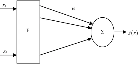
The structure of Chebyshev neural network (CNN) is shown in Figure 1 CNN is a functional link network (FLN) based on Chebyshev polynomials. There are two main parts in the architecture of CNN, namely, numerical transformation part and learning part. Numerical trans- formation deals with input to hidden layer by approxi- mate transformable method. The transformation is a functional expansion (FE) of input pattern comprising of a finite set of Chebyshev polynomials. As a result the Chebyshev polynomials basis can be viewed as a new input vector. The learning part is a functional-link neural network based on Chebyshev polynomials [30-33]. The Chebyshev polynomials can be obtained by a recursive formula
1 2 1 , 0 1
i i i
T x xT x T x T x (1)
where, i
are Chebyshev polynomials, i is the orderof polynomials chosen and here x is a scalar quantity. The different choices of
T x
1
The output of single layer neural network is given by
T x
ˆ( ) ˆT
are x & 2x.
g x w w
(2)
where, are the weights and is the suitable basis function of neural network. Based on the approximation property of CNN [30-33], there exist ideal weights w, so that the function g x
Tg x w
to be approximated can be rep-resented as
(3)
where, is the CNN functional reconstruction error vector and N is bounded.
Approximation of complex nonlinear systems becomes easier as CNN is a single layer neural network.
F x1
x2
w
[image:2.595.311.540.614.724.2] g x
3. Problem Formulation
Consider the discrete-time nonlinear system with a fixed known delay [25]
1
d
x k Ax k A x kh
g x k u k (4)
where, x k
Rn ( ) mu k R
and denote the state and input vectors respectively at time instant k. A and Ad
are constant matrices of appropriate dimensions.
g x k is a unknown nonlinear function of a given
system in (4), and h is a positive known number repre-senting delay.
For the system (4) the stabilizing controller is chosen as
2
2 ˆu k Ax k
g x k
1 A x kd
h
ˆ
(5)
where g x k
is the approximated value of unknown system function g x kˆ
. Let us assume g x kˆ
0w
. The objective of the current work is to ensure the sta-bility and performance of the nonlinear system (4), using the controller (5) and appropriate Lyapunov-Krasovskii functional (11).
4. Stability Analysis
For the stability analysis, the following assumptions are needed to proceed.
Assumption 1:(Bounded Ideal NN Weights): The ideal NN weights are bounded so that wF wM, with
M
w a known bound. The symbol ·F denotes the Fro-benius norm, i.e. given a matrix A, the Frobenius norm is given by [34],
2 T
F tr A
A A
Assumption 2: Let g x k
Gg x kˆ
T
GG
, where is a n n symmetric matrix, and g x k
and g x kˆ
are the n-column vectors. Equation (4) can be rewritten as
1 ˆ d
x k Ax k A x k h
g x k u k
g x k u k
(6) where
ˆ
g x k g x k g x k
n n
n n
(7)
The main results are as follows:
Theorem 1:
Suppose there exist an positive-definite matrix
P, an n n nonnegative-definite matrix Q, and symmetric matrix G such that following LMIs holds,
H1) T
A PA A
A P P Q 0 T T d d d PA A
Q (8)
and
H2) 0
T T T T
d d
T T
d d d d
A A A A A A A
A A A A
A
(9)
where PG and G PGT
then, the nonlinear d elay system (4) ensures the stability the control law in (5) and weight tuning algorithm
iscrete-time d with
12ˆ 1 ˆ T T
w k w k x k A PA x k
Q P
1 2 1 2 1 2 T T d d T T d T T dx k h A PA x k h
x k h A PA x k
x k A PA x k h
Q .(10) Proof:
Choose Lyapunov-Krasovskii functional,
1
2
3
V k V k V k V k (11) where,
1
T
V k x k Px k
1
2
k T
i k h
V k x i Qx i
(13) (12)
3
T
V k tr w k w k (14) Substituting (12)-(14) in (11)
1
k
T T
i k h
V k x k Px k x
k
(15) and
+1+1 +1 +1
+1 +1
k
T T
i k h T
V k x k Px k x i Qx i
tr w k w k
(16)Since P is a positive-definite and Q is a no tive-definite,
i Qx i
Ttr w k w
nnega-
V k is then positive-definite [25]. fore,
There-
1
V k V k V k
(17)
Substituting (15) and (16) in (17),
1 1 1 k T T h T k T Ti k h
V k x k Px k x
x k Px k
x i Qx i tr w k w k
(18)
i Qx i
1 1
+1i k T
tr w k w k
Substituting (6) in (18),
ˆ ˆ 1 1 h h d T d T T T T V kAx k A x k h g x k u k
g x k u k P Ax k A x k h
T
g x k u k g x k u k
x k Qx k tr w k w k
x k Qx k tr w k w k
x k Px k
(19) Using Assumption 1 in (19) and further solving (19),
ˆ ˆT T T T
d
T T T T
d
T T
T T
T T
Z k
x k A Pg x k u k x k h A Pg x k u k u k g x k PAx k u k g x k PA x k h u k g x k Pg x k u k
u k g x k Pg x k u k u k g x k Pg x k u k
(21) In (20) collecting the terms together, substitute control law from (5), adding and subtracting some terms to make perfect square yields,
2
2 T d T T d T T T T d T T T T T V kx k A PA x k x k A PA x k h
ˆ ˆ ˆ ˆ ˆ ˆ 1T T T T
d
T T T
T T
d d
x k A Pg x k u k x k h A PA x k
x k h A Pg x k u k
u k g x k PAx k
u k g x k PA x k h
u k g x k Pg x k u k
Z k x k Qx k x k Px k
x k h Qx k h w k w k
(20) where,
x k h A PA x k h
2 1 2 1 2 1 2 2 1 2 ˆ 1ˆ T T
T T d d T T d T T d V k w k
w k x k A PA Q P x k
x k h A PA Q x k h
x k h A PA x k
x k A PA x k h S k Z k
(22)
where, S k
is given in (23).
From (22) the weight tuning law is obtained as (24),
1 1 2 2 1 1 2 21 1 1
2 2 2
ˆ 2 T T d d T d d
T T T T T T
d d d
T T
S k w k x k A PA Q P x k x k h A PA Q x k h
x k h A PA x k x k x k h
w k x k A PA Q P x k x k h A PA Q x k h x k h A PA x k
w k x k A PA
ˆ 2 ˆ 2 T TT T T
A PA
1 1 2 2 1 2 ˆ 2 T T d d T TQ P x k x k h A PA Q x k h
w k x k A PA Q P x k
(23
)
1 1 2 2 1 1 2 2T T T T
d d
T T T T
d d
x k A PA Q P x k x k h A PA Q x k h
h A PA x k x k A PA x k h
ˆ 1 ˆ
w k w k
then (22) becomes,
S k Z k (25)
Substituting (5), (21) and (23) in (25), gives (26). Using Assumption 2,(26) is given by (27).
V k
1 1 2 2 1 1 2 1 2 1 1 2 2 ˆ 2 ˆ 2 ˆ 2T T T T
d d
T T T
d d
T T
T T T T
d d d
T T
V k w k x k A PA Q P x k x k h A PA Q x k h
k h A PA x k x k A PA x
w k x k A PA Q P x k
x k h A PA Q x k h x k h A PA x k
w k x k A PA
2kh
T x
1 1 2 2 1 2 1 ˆ2 2 2 2
ˆ
1
2 2 2
ˆ
1
2 2 2
ˆ
T T
d d
T T T T
d T T d d T T d
Q P x k x k h A PA Q x k h
w k x k A PA Q P x k x k A Pg x k Ax k A x k h
g x k
x k h A Pg x k Ax k A x k h
g x k
Ax k A x k h g x k P
g x k
1ˆ 2 2
ˆ
1 1
2 2 2 2
ˆ ˆ
d
T T
d d
g x k Ax k A x k h
g x k
Ax k A x k h g x k Pg x k Ax k A x k h
g x k g x k
(26)
1 1 2 2 1 1 2 2 2 2 2T T T T
d
T T T T
d
T T
d d
x k A PA Q P x k x k A PA x k h
x k A PA Q P x k x k h A PA x k
x k h A PA Q x
1 1 2 2 1 1 2 2 ˆ ˆ 2 2 ˆ ˆ 2 2T T T T
d d
T T T T
d d
V k w k x k A PA x k h w k x k h A PA x k
w k x k h A PA Q x k h w k x k A PA Q P x k
1 1 2 2 1 1 2 2 1 1 2 2 1 1 2 2 2 2 24 4 4 4
T T
d
T T T T
d d d
T T T T
d d
T T T T
d d
T T T T T T T T
d d
k h x k A PA x k h
x k h A PA Q x k h x k h A PA x k
x k h A PA x k x k A PA x k h
x k A PA Q P x k x k h A PA Q x k h
x k A PGA A G PGA x k x k A PGA A G PGA x
4 4
4 4T T T T T T T
d d d d d
k
T d hx k h A PGA A G PGA x k x k h A PGA A G P
GA x k h
(27)
Let,
1 1 2 2 1 1 2 2 1 1 2 2 1 1 2 2T T T T
d
T T T T
d T
T d
a x k A PA Q P x k x k A PA x k h
PA x k
A x k
A x k h
Manipu lowing in d d
T T T
d d
T T T
d d
c
b x k h A PA Q x k h x k h A
x k A PA Q P x k x k h A P
d x k h A PA Q x k h x k A P
lating the nonquadratic terms using the fol-equality
2
a b
ab
(which turns into equality if and only if a = b) we get (28). In (28), V k
is guaranteed to remain negative as long as 0 T T d T d dA PA P Q A PA
A PA Q
and 0
T T T T
d d
T T
d d d d
A A A A A A A A
A A A A
where PG and G PT G.
Since in (28) the first four quadratic terms are negative, next four terms are satisfying LMI in (8), and remaining last four terms are satisfying LMI in (9). Therefore, we can conclude that the system (4) is stable with control law (5) and two LMIs in (8) and (9).
5. Simulation Results
A numerical example is presented to demonstrate the performance and the effectiveness of the proposed scheme.
Consider the non-linear discrete-time delay sy with the following parameters [25]:
0.8 0.4 0.2 0
0.14 0.1 d 0 0.1
stem (4)
A , A
and
1 1 2 2 11 1 2
2 2 1 2 1 1 2 2 4 2
T T T T
d
T T T T
d d d
T T T
T T
d
A PA Q P x k x k A PA x k h
x k h A PA Q x k h x k h A PA x k
x k A PA Q P x k x
x k A PA x k h
x k h A PA
1 2 1 2 T d T Tk h A PA x k
4
V k x k
T T
x kh A PAd dQ x k h d
1 1 2 1 1 2 2 1 1 2 2 1 1 2 2 2 ˆ 2 ( )4 4 4
T
T T T
T T
F d d
T T T T
d d
T T T T T T
d
x k x k A
x k A PA Q P x k x
w k x k A PA x k h
h A PA Q x k h A PA Q P x k
x k A PGA A G PGA x k x k A PGA
44 4 4 4
T T d
T T T T T T T T
d d d d d d
A G PGA x k h
2
T d
T
PA x k h
k h A
d d
T T
PA Q x k h
x k h A PA x k
x k x k
x k h A PGA A G PGA x k x k h A PGA A G PGA x k h
2 1 2 1
1
2 2
1 2
x k
x k
x k
1.4 1
1
g x k
x k x k
The delay time to be h2. The initial con-
di on of 1
is assumed
ti states x and x2 are chosen are solved
0.01 0.02
T.e LMIs n H1) by using Matlab
LMI Toolbox and the values ofP, Q & G are obtained,
6 0.1492 0.6183 10
0.6183 2.6654
Th i and H2)
P
25.7298 59.1751 59.1751 132.4626
Q
0.1707 0.0546 , 0.0546 0.7737
G
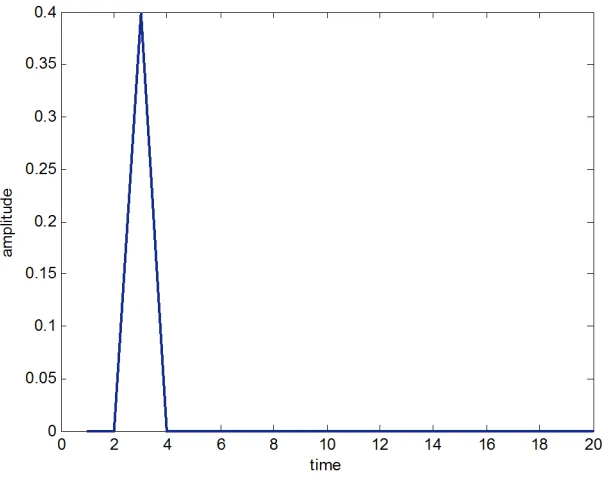
[image:7.595.110.237.84.154.2]Figures 2 and 3 show the responses of state variables
Figure 2. x1(k) with respect to sample time k (h = 2).
Figure 3. x2(k) with respect to sample time k (h = 2).
[image:7.595.371.478.85.189.2]Figure 4. u(k) with respect to sample time k (h = 2).
1
x and x2. Figure 4 displays the control input signal. Clearly, simulation results verify our theoretical findings and show the effectiveness of proposed scheme.
6. Conclusion
In this paper the problem of stabilization in discrete-time delay nonlinear system is studied, where the system dy-namics is assumed to be unknown. The unknown non- linear functions of the system are approximated through CNN. Two LMIs derived here are sufficient to charac- terize the controller, which ensures the stability for the resulting closed loop system. A numerical example, with fixed known delay, has been provided to demonstrate the effectiveness and the applicability of the proposed ap- proach.
REFERENCES
[1] M. Basin, J. Perez and R. Martinenz-Zuniga, “Optimal Filtering for Nonlinear Polynomial Systems over Linear Observations with Delay,” Inter
novative Computing Information and Control, Vol. 2, 2006, pp. 863-874.
[2] J. Chen, D. M. Xu and B. Shafai, “On Sufficient Condi-tions for Stability Independent of Delay,” IEEE Transac-tions on Automatic Control, Vol. 40, No. 9, 1995, pp. 1675-1680. doi:10.1109/9.412644
national Journal of
In-[3] E. Fridman and U. Shaked, “Stability and Guaranteed Cost Control of Uncertain Discrete-Delay Systems,” In-ternational Journal of Control, Vol. 78, No. 4, 2005, pp. 235-246. doi:10.1080/00207170500041472
[4] C. Lin, Q.-G. Wang and T. H. Lee, “A Less Conservative Robust Stability Test for Linear Uncertain Time-Delay
Systems,” IEEE Transactions on Automatic Control, Vol. 51, No. 1, 2006, pp. 87-91.
doi:10.1109/TAC.2005.861720
[5] Z. Wang, B. Huang and H. Unbehauen, “Robust Hx Ob-
server Design of Linear State Delayed Systems with Pa- rameteric Uncertainty: The Discrete-Time Case,” Auto- matica, Vol. 35, No. 6, 1999, pp. 1161-1167.
doi:10.1016/S0005-1098(99)00008-4
[6] Y. He, Q. G. Wang, C. Lin and M. Wu, “Delay-Range- Dependent Stability for Systems with Time Varying De- lay,” Automatica, Vol. 43, No. 2, 2007, pp. 371-376. doi:10.1016/j.automatica.2006.08.015
[7] X. Li and C. de Sauza, “Criteria for Robust Stability and Stabilization of Uncertain Linear Systems with State De- lay,” Automatica, Vol. 33, No. 9, 1997, pp. 1697-1662. doi:10.1016/S0005-1098(97)00082-4
[8] V. Kolmanvoskii and J.-P. Richard, “Stability of Some Linear Systems with Delays,” IEEE Transactions on Automatic Control, Vol. 44, No. 5, 1999, pp. 984-989. doi:10.1109/9.763213
[9] E. Fridman, “New Lyapunov-Kr ovskii Functional for Stability of Linear Retarted and utral Type Systems,” l Letters, Vol. 43, No. 4, 2001, pp. 309-319. doi:10.1016/S0167-6911(01)00114-1
as Ne Systems and Contro
[10] S.-I. Niculescu, “Delay Effects on Stability: A Robust Control Approach,” Lecture Notes in Control and Infor- mation Sciences, Vol. 269, Springer-Verlag, London, 2001.
[11] E. Fridman and U. Shaked, “An Improved Stabilization Method for Linear Systems with Time-Delay,” IEEE Tran- sactions on Automation Control, Vol. 47, No. 11, 2002, pp. 1931-1937. doi:10.1109/TAC.2002.804462
[image:8.595.146.450.83.326.2]5-9 July 2004.
[13] K. J. Astrom and B. Wittenmark, “Computer Controlled Systems: Theory and Design,” Prentice-Hall Inc., Engle-wood Cliffs, 1984.
[14] E. Fridman and U. Shaked, “An LMI Approach to Stabil-ity of Discrete Delay Systems,” Proceedings of 7th IEE European Control Conference, Cambridge, 1-4 Septem-ber, 2003.
[15] Y. S. Lee and W. H. Kwon, “Delay Dependent Robust Stabilization of Uncertain Discrete-Time State-Delayed Systems,” 15th Triennial World Congress, Barcelona, 21-26 July 2002.
[16] S. S. Ge, F. Hong and T. H. Lee, “Adaptive Neural Net- work Control of Nonlinear Systems with Unknown Time Delays,” IEEE Transactions on Automatic Control,Vol. 48, No. 11, 2003, pp. 2004-2010.
doi:10.1109/TAC.2003.819287
[17] S. S. Ge, F. Hong and T. H. Lee, “Adaptive Neural Con- trol of Nonlinear Time-Delay Systems with Unknown Virtual Control Coefficients,” IEEE Transactions on Sys- tems, Man, and Cybernetics—Part B: Cybernetics, Vol. 34, No. 1, 2004, pp. 499-516.
doi:10.1109/TSMCB.2003.817055
[18] D. W C. Ho, J. Li and Y. Niu, “Adaptive Neural Control for a Class of Nonlinearly Parametric Time-Delay Sys- tems,” IEEE Transactions on Neural Networks,Vol. 16, No. 3, 2005, pp. 625-635.
.
.844907 doi:10.1109/TNN.2005
a [19] A. Kulkarni an
Class of Dela
d S. Purwar, “Backstepping Control for yed Nonlinear Systems with Input Con-straints,” IEEE Conference, Vol. 1, 2008, pp. 274-279. [20] B. Chen, X. P. Liu, K. F. Liu and C. Lin, “Fuzzy-Ap-
proximation-Based Adaptive Control of Strict-Feedback Nonlinear Systems with Time Delays,” IEEE Transac- tions on Fuzzy Systems,Vol. 18, No. 5, 2010, pp. 883-891. doi:10.1109/TFUZZ.2010.2050892
[21] W. Aggoune, R. Kharel and K. Busawon, “On Feedback Stabilization of Nonlinear Discrete-Time State-Delayed Systems,” ECC Conference, Budapest, 23-26 August 2009.
[22] H. J. Gao and T. W. Chen, “New Results on Stabili Discrete-Time Systems with Time-Varying State Delay,” IEEE Transac rol,Vol. 52, No. 2, 2007, pp. 328- 006.890320
ty of tions on Automatic Cont
334. doi:10.1109/TAC.2
20600774289
[23] S. Ibrir, W. F. Xie and C.-Y. Su, “Observer Design for Discrete-Time Systems Subject to Time Delay Nonlin- earities,” International Journal of Systems Science, Vol. 37, No. 9, 2006, pp. 629-641.
doi:10.1080/002077
Optimal Control Scheme for a Class of Discrete-Time Nonlinear Systems with t Delays Using Adaptive Dy- namic Programming,” ACTA Automatica Sinica,Vol. 36, No. 1, 2010, pp. 121-129.
doi:10.3724/SP.J.1004.2010.00121
[25] K. E. Bouazza, M. Boutayeb and M. Darouach, “State Feedback Stabilization of Discrete-Time Delay Nonlinear Systems,” Proceedings of Mathematical Theory of Net- works and Systems,Leuven, 5-9 July 2004.
[26] E. J. Hartman, J. D. Keelar and J. M. Kowalski, “Layered Neural Networks with Gaussian Hidden Units as Univer- sal Approximation,” Neural Computation, Vol. 2, 1990, pp. 210-215. doi:10.1162/neco.1990.2.2.210
[27] S. Chen, S. A. Billings and P. M. Grant, “Recursive Hy- brid Algorithm for Nonlinear System Identification Using Radial Basis Function Networks,” International Journal of Control, Vol. 55, No. 5, 1992, pp. 1051-1070. doi:10.1080/00207179208934272
[28] S. V. T. Elanayar and Y. C. Shin, “Radial Basis Function Neural Network for Approximation and Estimation of Nonlinear Stochastic Dynamic S tems,” IEEE Transac- tions on Neural Networks, Vol. No. 4, 1994, pp. 594-
.298229
[24] Q.-L. Wei, H.-G. Zhang, D.-R. Liu and Y. Zhao, “An
ys 5, 603. doi:10.1109/72
actions on Systems, Man, 2002, pp. 505-511. [29] J. C. Patra and A. C. Kot, “Nonlinear Dynamic System
Identification Using Chebyshev Functional Link Artificial Neural Networks,” IEEE Trans
and Cybernetics, Vol. 32, No. 4, doi:10.1109/TSMCB.2002.1018769
[30] A. Namatame and N. Ueda, “Pattern Classification with Chebyshev Neural Network,” International Journal Neu- ral Network, Vol. 3, 1992, pp. 23-31.
[31] T. T. Lee and J. T. Jeng, “The Chebyshev Polynomial Based Unified Model Neural Networks for Functions Approximations,” IEEE Transactions on Systems, Man & Cybernetics, Part B,Vol. 28, No. 6, 1998, pp. 925-935. [32] S. Purwar, I. N. Kar and A. N. Jha, “Adaptive Output
Feedback Tracking Control of Robot Manipulators Using Position Measurements Only,” Expert Systems with Ap-plications, Vol. 34, No. 4, 2008, pp. 2789-2798. doi:10.1016/j.eswa.2007.05.030
[33] S. Purwar, I. N. Kar and A. N. Jha, “On-Line System Identification of Complex Systems Using Chebyshev Neural Networks,” Applied Soft Computing, Vol. 7, No. 2005, pp. 364-372. doi:
1, 10.1016/j.asoc.2005.08.001
[34] C. Kwan and F. L. Lewis, “Robust Backstepping Control of Nonlinear Systems Using Neural Networks,” IEEE Transactions on Systems, Man, and Cybernetics, Vol. 30, No. 6, 2000, pp. 753-766. doi:10.1109/3468.895898