Authorship Attribution with Topic Models

Yanir Seroussi

Ingrid Zukerman

Fabian Bohnert

Authorship attribution deals with identifying the authors of anonymous texts. Traditionally, research in this field has focused on formal texts, such as essays and novels, but recently more attention has been given to texts generated by on-line users, such as e-mails and blogs. Authorship attribution of such on-line texts is a more challenging task than traditional author-ship attribution, because such texts tend to be short, and the number of candidate authors is often larger than in traditional settings. We address this challenge by using topic models to obtain author representations. In addition to exploring novel ways of applying two popular topic models to this task, we test our new model that projects authors and documents to two disjoint topic spaces. Utilizing our model in authorship attribution yields state-of-the-art performance on several data sets, containing either formal texts written by a few authors or informal texts gener-ated by tens to thousands of on-line users. We also present experimental results that demonstrate the applicability of topical author representations to two other problems: inferring the sentiment polarity of texts, and predicting the ratings that users would give to items such as movies.

1. Introduction

Authorship attribution has attracted much attention due to its many applications in, for example, computer forensics, criminal law, military intelligence, and humanities research (Juola 2006; Stamatatos 2009; Argamon and Juola 2011). The traditional prob-lem, which is the focus of this article, is to attribute anonymous test texts to one of a set of known candidate authors, whosetraining texts are supplied in advance (i.e., supervised classification). Whereas most of the early work on authorship attribution focused on formal texts with only a few candidate authors, researchers have recently

∗Faculty of Information Technology, Monash University, Clayton, Victoria 3800, Australia. E-mail:[email protected].

∗∗Faculty of Information Technology, Monash University, Clayton, Victoria 3800, Australia. E-mail:[email protected].

†Faculty of Information Technology, Monash University, Clayton, Victoria 3800, Australia. E-mail:[email protected].

Submission received: 30 December 2012; revised submission received: 9 May 2013; accepted for publication: 23 June 2013.

turned their attention to scenarios involving informal texts and tens to thousands of authors (Koppel, Schler, and Argamon 2011; Luyckx and Daelemans 2011). In parallel, topic models have gained popularity as a means of discovering themes in such large text corpora (Blei 2012). This article explores authorship attribution with topic models, extending the work presented by Seroussi and colleagues (Seroussi, Zukerman, and Bohnert 2011; Seroussi, Bohnert, and Zukerman 2012) by reporting additional experi-mental results and applications of topic-based author representations that go beyond traditional authorship attribution.

Topic models work by defining a probabilistic representation of the latent structure of corpora through latent factors called topics, which are commonly associated with distributions over words (Blei 2012). For example, in the popular Latent Dirichlet Allocation (LDA) topic model, each document is associated with a distribution over topics, and each word in the document is generated according to its topic’s distribution over words (Blei, Ng, and Jordan 2003). The word distributions often correspond to a human-interpretable notion of topics, but this is not guaranteed, as interpretability depends on the corpus used for training the model. Indeed, when we ran LDA on a data set of movie reviews and message board posts, we found that some word distributions correspond to authorship style as reflected by authors’ vocabulary, with netspeak words such as “wanna,” “alot,” and “haha” assigned to one topic, and words such as “compelling” and “beautifully” assigned to a different topic. This finding motivated our use of LDA for authorship attribution (Seroussi, Zukerman, and Bohnert 2011).

One limitation of LDA is that it does not model authors explicitly. This led us to use Rosen-Zvi et al.’s (2004) Author-Topic (AT) model to obtain improved authorship attribution results (Seroussi, Bohnert, and Zukerman 2012). However, AT is also limited in that it does not model documents. We addressed this limitation through the Disjoint Author-Document Topic (DADT) model—a topic model that draws on the strengths of LDA and AT, while addressing their limitations by integrating them into a single model. Our DADT model extends the model introduced by Seroussi, Bohnert, and Zukerman (2012), which could only be trained on single-authored texts. In this article, we provide a detailed account of the extended model. In addition, we offer experimental results for five data sets, extending the results by Seroussi, Bohnert, and Zukerman (2012), which were restricted to two data sets of informal texts with many authors. Our experiments show that DADT yields state-of-the-art performance on these data sets, which contain either formal texts written by a few authors or informal texts where the number of candidate authors ranges from 62 to about 20,000.

Although our evaluation is focused on single-authored texts, AT and DADT can also be used to model authors based on multi-authored texts, such as research papers. To demonstrate the potential utility of this capability of the models, we present the results of a preliminary study, where we use AT and DADT to identify anonymous reviewers based on publicly available information (reviewer lists and the reviewers’ publications, which are often multi-authored). Our results indicate that reviewers may be identified with moderate accuracy, at least in small conference tracks and workshops. We hope that these results will help fuel discussions on the issue of reviewer anonymity.

showing how topic models can be utilized to improve the performance of methods we developed to address the popular tasks of polarity inference and rating prediction.

This article is structured as follows. Section 2 surveys related work. Section 3 discusses LDA, AT, and DADT and the author representations they yield. Section 4 introduces authorship attribution methods, which are evaluated in Section 5. Section 6 presents applications of our topic-based approach, and Section 7 concludes the article.

2. Related Work

Authorship attribution has a long history that predates modern computing. For exam-ple, Mendenhall (1887) suggested that word length can be used to distinguish works by different authors. Modern interest in authorship attribution is commonly traced back to Mosteller and Wallace’s (1964) study on applying Bayesian statistical analysis of function word frequencies to uncover the authors of theFederalist Papers (Juola 2006; Koppel, Schler, and Argamon 2009; Stamatatos 2009). The interest in authorship attri-bution is due to its many applications in areas such as computer forensics, criminal law, military intelligence, and humanities research. In recent years, authorship attribution research has been fuelled by advances in natural language processing, text mining, machine learning, information retrieval, and statistical analysis. This has motivated the organization of workshops and competitions to facilitate the development and comparison of authorship attribution methods (Juola 2004; Argamon and Juola 2011).

In this article, we focus on the closed-setattribution task, where training texts by the candidate authors are supplied in advance, and for each test text, the goal is to attribute the text to the correct author out of the candidate authors (Argamon and Juola 2011). Related tasks includeopen-setattribution, where some test texts may not have been written by any of the candidate authors, andverification, where texts by only one candidate author are supplied in advance, and the task is to verify whether test texts were written by the candidate author (Koppel and Schler 2004; Sanderson and Guenter 2006; Koppel, Schler, and Argamon 2011).

Regardless of the task, a challenge currently faced by researchers in the field is addressing scenarios with many candidate authors and varying amounts of data per author (Argamon and Juola 2011; Koppel, Schler, and Argamon 2011; Luyckx and Daelemans 2011). This challenge is illustrated by the corpus chosen for the PAN’11 competition (Argamon and Juola 2011), which contains short e-mails by tens of authors. Other examples are Koppel, Schler, and Argamon’s (2011) work on a corpus of blog posts by thousands of authors, and Luyckx and Daelemans’s (2011) study of the effect of the number of authors and training set size on authorship attribution performance on data sets of student essays. Our approach to authorship attribution addresses this challenge by using topic models, which are known to successfully deal with varying amounts of text (Blei 2012).

because an author’s native language may manifest itself in only a few words, or maybe due to data-set-specific issues), Pearl and Steyvers found that topical representations helped them achieve state-of-the-art verification accuracy. Pearl and Steyvers’s findings further strengthen our hypothesis that topic models yield meaningful author representations. We take this observation one step further by defining our DADT model, and applying it to several authorship attribution scenarios, where it yields better performance than LDA-based approaches and methods based on the AT model (Section 5).

A line of research that has garnered much interest in recent years is the definition of generic topic models that incorporate metadata labels (Blei 2012). These models can be divided into two types: upstream models, which use the labels to constrain the topics, and downstream models, which generate the labels from the topics (Mimno and McCallum 2008). Generic models have the appealing advantage of obviating the need to define a new model for each new task (e.g., they may be used to obtain author representations by defining a metadata label for each author). However, this advantage may come at the price of increased computational complexity or poorer performance than that of task-specific models (Mimno and McCallum 2008). As the focus of our work is on modeling authors, we experimented only with LDA and with the task-specific topic models discussed in Section 3 (AT and DADT, which model authors explicitly). The applicability of generic models to authorship attribution is an open question that would be interesting to investigate in the future. Nonetheless, most of the generic models surveyed here have properties that make them unsuitable for our purposes.

Examples of generic upstream models include DiscLDA (Lacoste-Julien, Sha, and Jordan 2008), Labeled LDA (Ramage et al. 2009), and DMR (Mimno and McCallum 2008). The former two dedicate at least one topic to each metadata label, making them too computationally expensive to use on data sets with thousands of authors, such as the Blog and IMDb1M data sets (Section 5.1). In contrast to DiscLDA and Labeled LDA, DMR uses less topics by sharing them between labels. Mimno and McCallum (2008) showed that DMR outperformed AT on authorship attribution of multi-authored documents. Despite this, we decided to use AT, because we found in preliminary exper-iments that AT performs better than DMR on authorship attribution of single-authored texts. Such texts are the main focus of this article. Nonetheless, it is worth noting that Mimno and McCallum’s experiments were performed on a data set of research papers where stopwords were filtered out. We do not discard stopwords in most experiments, because they are known to be indicators of authorship (Koppel, Schler, and Argamon 2009).1

A representative example of a generic downstream model is sLDA (Blei and McAuliffe 2007), which generates labels from each document’s topic assignments via a generalized linear model. This model was extended by Zhu, Ahmed, and Xing (2009), who introduced MedLDA, where training is done in a way that maximizes the margin between labels, which is “arguably more suitable” for inferring document labels. Zhu

and Xing (2010) further extended that work by introducing sCTRF, which combines sLDA with conditional random fields to accommodate arbitrary types of features. Zhu and Xing applied these models to the polarity inference task, and found that support vector regression outperformed sLDA and performed comparably to MedLDA (these three models used only unigrams), whereas sCTRF yielded the best performance by incorporating additional feature types (e.g., part-of-speech tags and a lexicon of positive and negative words). Based on these results, we decided to leave experiments with downstream models for future work, as it seems unlikely that we would obtain good results on the authorship attribution task without considering other feature types in addition to token unigrams (which is beyond the scope of this article).

3. Topic Models and Author Representations

This section introduces notation, provides a discussion of the meaning of the parameters used by the topic models, and describes the three topic models considered in this article (LDA, AT, and DADT), focusing on the author representations that they yield.

3.1 Notation and Preliminaries

We denote matrices and stacked vectors in uppercase boldface italics (e.g.,MMM), and vectors in lowercase boldface italics (e.g.,vvv). The element at thei-th row andj-th column of a matrixMMMis denotedmij, and vector elements are denoted in lowercase italics with

a subscript index (e.g.,vi). Sets are denoted with calligraphic font (e.g.,S). In addition,

Dir and Cat denote the Dirichlet and categorical distributions, respectively.

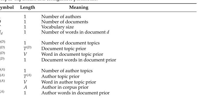
The values of the parameters that are given as input to the models are either deter-mined by the corpus (Section 3.1.1) or configured when using the models (Sections 3.1.2 and 3.1.3). Table 1 shows the models’ corpus-dependent and configurable parameters with their lengths and meanings (scalars have length 1). Corpus-dependent parameters are at the top, configurable document-related parameters are in the middle (for LDA

Table 1

Corpus-dependent and configurable parameters.

Symbol Length Meaning

A 1 Number of authors

D 1 Number of documents

V 1 Vocabulary size

Nd 1 Number of words in documentd

T(D) _{1 Number of document topics}

α

αα(D) T(D) Document topic prior βββ(D) V Word in document topic prior δ(D) 1 Document words in document prior

T(A) _{1 Number of author topics}

α

αα(A) T(A) Author topic prior βββ(A) V Word in author topic prior η

ηη A Author in corpus prior

and DADT), and configurable author-related parameters are at the bottom (for AT and DADT).

3.1.1 Corpus-Dependent Parameters. The following parameters depend on the corpus, and are thus considered to be observed:

A: Number of authors. We usea∈ {1,. . .,A}to denote an author identifier.

D: Number of documents. We used∈ {1,. . .,D}to denote a document identifier.

V: Vocabulary size. We usev∈ {1,. . .,V}to denote a unique word identifier.

Nd: Number of words in documentd. We usei∈ {1,. . .,Nd}to denote a word index

in documentd.

AAA: Document authors. This is a D-dimensional vector of vectors, where the d-th elementaaad contains the authors of thed-th document. In cases where the corpus

contains only single-authored texts, we use the scalarad to denote the author of

thed-th document, sinceaaadis always of unit length.

W W

W: Document words. This is a D-dimensional vector of vectors, where the d-th elementwwwdcontains the words of thed-th document. The vectorwwwdis of lengthNd,

andwdi ∈ {1,. . .,V}is thei-th word in thed-th document.

3.1.2 Number of Topics.We make a distinction betweendocumenttopics andauthortopics. In both cases, “topics” describe distributions over all the words in the vocabulary. The difference is that document topics are word distributions that arise from documents, while author topics are word distributions that characterize the authors. LDA uses only document topics, whereas AT uses only author topics. DADT, our hybrid model, uses both document topics and author topics.

All three models take the number of topics as a configurable parameter, denoted by T(D) for the number of document topics and by T(A) for the number of author topics. Although the models have other configurable parameters (introduced subse-quently), we found that the number of topics has the largest impact on model perfor-mance because it controls the overall model complexity. For example, settingT(D)=1 in LDA means that all the words in all the documents are drawn from the same topic (i.e., a single distribution for all the words), whereas settingT(D)=200 gives LDA much more freedom to adapt to the corpus, as each word can be drawn from one of 200 distributions.

It is worth noting that techniques for determining the optimal number of topics have been suggested. For example, Teh et al. (2006) used hierarchical Dirichlet processes to learn the number of topics while inferring the LDA model. We did not experiment with such techniques as they tend to complicate model inference, and we found that using a constant number of topics yields good performance. Nonetheless, we note that utilizing such techniques may be a worthwhile future research direction, especially to determine the balance between document topics and author topics for DADT.

The priors are defined as follows (all vector elements and scalars are positive):

α

αα(D): Document topic prior – a vector of lengthT(D). β

β

β(D): Prior for words in document topics – a vector of lengthV. α

α

α(A): Author topic prior – a vector of lengthT(A).

βββ(A): Prior for words in author topics – a vector of lengthV. δ(D): Document words in document prior.

δ(A): Author words in document prior. η

η

η: Author in corpus prior – a vector of lengthA.

The support of a K-dimensional Dirichlet distribution Dir(ααα) is the set of K

-dimensional vectors with elements in the range [0, 1] whose sum is 1 (the Dirichlet distribution is a multivariate generalization of the beta distribution). Hence, each draw from the Dirichlet distribution can be seen as defining the parameters of a categorical distribution. This is illustrated by Figure 1, which shows the Dirichlet distribution density in the three-dimensional case for three different prior vectorsααα (the density

is triangular because the drawn vector elements have to sum to 1—each corner of the triangle corresponds to a dimension of the distribution, denoted 1, 2, and 3 in Figure 1). When the prior vector is symmetric (i.e., all its elements have the same value), the density is also symmetric (Figures 1a and 1b). Symmetric priors with element values that are greater than 1 yield densities that are concentrated in the middle of the triangle, meaning that categorical vectors with relatively uniform values are likely to be drawn (Figure 1a). On the other hand, symmetric priors with element values that are less than 1 yield sparse densities with high values in the corners of the triangle, meaning that the categorical vectors are likely to have one element whose value is greater than the other elements (Figure 1b). Finally, when the prior is asymmetric, vectors that give higher probabilities to the elements with higher prior values are likely to be drawn (Figure 1c).

The document and author topic priors (ααα(D) and ααα(A), respectively) encode our

beliefs about the document and author topic distributions, respectively. They are often set to be symmetric, because we have no reason to favor one topic over the other before we have seen the data (Steyvers and Griffiths 2007). Wallach, Mimno, and McCallum (2009) argue that using asymmetric priors in LDA is beneficial, and suggest a method that learns such priors as part of model inference (by placing another prior on theααα(D)

prior). We implemented Wallach, Mimno and McCallum’s method for all the models we considered, but found that it did not improve authorship attribution accuracy in preliminary experiments. Thus, in all our experiments we set the elements of ααα(D)

and ααα(A) to min{0.1, 5/T(D)} and min{0.1, 5/T(A)}, respectively, yielding relatively

sparse topic distributions, since we expect each document and author to be sufficiently

1

2 3

1

2 3

1

2 3

High

Low

(a)ααα= (2, 2, 2) (b)ααα= (0.5, 0.5, 0.5) (c)ααα= (0.9, 0.5, 0.5)

Figure 1

represented by only a few topics. This choice follows the recommendations from LingPipe’s documentation (alias-i.com/lingpipe), which are based on empirical evidence from several corpora.

The priors for words in document and author topics (βββ(D) andβββ(A), respectively)

encode our beliefs about the word distributions. As for the topic distribution priors, symmetric priors are often used, with a default value of 0.01 for all the vector ele-ments (yielding sparse word distributions, as indicated earlier), meaning that each topic is expected to assign high probabilities to only a few top words (Steyvers and Griffiths 2007). In contrast to the topic distribution priors, Wallach, Mimno, and McCallum (2009) found in their experiments on LDA that using an asymmetricβββ(D) was of no benefit.

This is because using an asymmetric βββ(D) means that we encode a prior preference

for a certain word to appear in all topics (e.g., a word represented by corner 1 in Figure 1c). For the same reason, using a symmetricβββ(A)is a sensible choice for AT. In

contrast to LDA and AT, our DADT model distinguishes between document words and author words, and thus uses bothβββ(D)andβββ(A)as priors. This allows us to encode our

prior knowledge that stopword use is indicative of authorship. Thus, for DADT we set

βv(D)=0.01−eandβv(A)=0.01+efor allv, wherevis a stopword (ecan be set to zero

to obtain symmetric priors).

DADT’s δ(D) and δ(A) priors encode our prior belief about the balance between

document words and author words in a given document. Document words (drawn from document topics) are expected to be representative of the documents in the corpus, whereas author words (drawn from author topics) characterize the authors in the corpus. For example, if we asked two different authors to write a report about LDA, both reports are likely to contain content words like Dirichlet,topic, and prior, but the frequencies of non-content words (i.e., function words and other indicators of authorship style) are likely to vary across the reports. In this case, the content words are expected to be allocated to document topics, and the non-content words whose usage varies across authors would be allocated to author topics. In cases where the authors write about different issues, DADT may allocate some content words to author topics (i.e., the meaning of DADT’s topics is expected to be corpus-specific). According to DADT’s definition (Section 3.4.1), which uses the beta distribution, the prior expected value of the portion of each document that is composed of author words is

δ(A)

δ(A)+δ(D) (1)

with a variance of

δ(A)δ(D)

δ(A)+δ(D)2 δ(A)+δ(D)+1

(2)

In our experiments, we chose values forδ(D)andδ(A)by deciding on the expected value

and variance, and solving these equations forδ(D)andδ(A).

Finally, DADT’sηηηprior determines the prior belief about an author having written a

w_di D N_d zdi

®

D

µ_d(D) (D)

¯

T

Á_t (D) (D) (D)

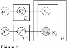
Figure 2

Latent Dirichlet allocation (LDA).

3.2 LDA

3.2.1 Model Definition.LDA was originally defined by Blei, Ng, and Jordan (2003). Here we describe Griffiths and Steyvers’s (2004) extended version. The idea behind LDA is that each document in a corpus is described by a distribution over topics, and each word in the document is drawn from its topic’s word distribution. Figure 2 presents LDA in plate notation, where observed variables are in shaded circles, unobserved variables are in unshaded circles, and each box represents repeated sampling, with the number of repetitions at the bottom-right corner. Formally, the generative process is: (1) for each topict, draw a word distributionφφφ_t(D)∼Dir βββ(D); (2) for each documentd, draw a topic

distributionθθθ(_dD)∼Dir ααα(D); and (3) for each word indexiin each documentd, draw a

topiczdi∼Cat (θθθ(_dD)), and the wordwdi ∼Cat (φφφ(zdiD)).

3.2.2 Model Inference.Topic models are commonly inferred using either collapsed Gibbs sampling (Griffiths and Steyvers 2004; Rosen-Zvi et al. 2004) or methods based on vari-ational inference (Blei, Ng, and Jordan 2003). We use collapsed Gibbs sampling to infer all models due to its efficiency and ease of implementation. This involves repeatedly sampling from the conditional distribution of the latent parameters, which is obtained analytically by marginalizing over the topic and word distributions, and using the prop-erties of conjugate priors. This conditional distribution is given in Equation (3) (Griffiths and Steyvers 2004; Steyvers and Griffiths 2007):

p zdi=t|WWW,ZZZ−di;ααα(D),βββ(D)∝ α

(D)

t +c

(DT)

dt

PT(D)

t0₌₁

α_t(D0)+c(_dtDT0 )

β(wDdi)+c

(DTV)

twdi

PV

v=1

β(vD)+c(tvDTV)

(3)

whereWWWis the corpus;ZZZ−di contains all the topic assignments, excluding the

assign-ment for thei-th word of thed-th document;c(_dtDT)is the count of topictin documentd; and c(_twdiDTV) is the count of word wdi in document topic t. Here, these counts exclude

thedi-th topic assignment (i.e.,zdi).

Commonly, several Gibbs sampling chains are run, and several samples are retained from each chain after a burn-in period, which allows the chain to reach its stationary distribution. For each sample, the topic distributions and the word distributions are estimated using their expected values, given the topic assignmentsZZZ. These expected values are given in Equations (4) and (5):

E[θ_dt(D)|ZZZ]= α

(D)

t +c

(DT)

dt

PT(D)

t0₌₁

α_t(D0)+c_dt(DT0 )

E[φ_tv(D)|ZZZ]= β

(D)

v +c(tvDTV)

PV

v0₌₁

β(_vD0)+c(_tvDTV0 )

(5)

where in this case the counts are over the full topic and author assignments. The two equations take a similar form due to the fact that the Dirichlet distribution is the conjugate prior of the categorical distribution (Griffiths and Steyvers 2004). Note that these values cannot be averaged across samples due to the exchangeability of the topics (Steyvers and Griffiths 2007) (e.g., topic 1 in one sample is not necessarily the same as topic 1 in another sample).

The examined authorship attribution problem follows a supervised classification setup, where training texts with known candidate authors are given in advance. Test texts are classified one by one, and the goal is to attribute each test text to one of the candidate authors. As the word distributions of the LDA model inferred in the training phase are unlikely to change much due to the addition of a single test document, in the classification phase we consider each topic’s word distribution to be observed, setting it to its expected value according to Equation (5). This yields the following sampling equation for a given test text ˜www˜˜ ( ˜www˜˜is a word vector of length ˜N):

p z˜i=t|www˜˜˜, ˜zzz˜˜−i;ΦΦΦ(D),ααα(D)∝ α

(D)

t +c˜

(DT)

t

PT(D)

t0₌₁

α(_t0D)+c˜(_t0DT)

φ

(D)

twi˜ (6)

where ˜zi is the topic assignment for the i-th word in ˜www˜˜, ˜zzz˜˜−i contains all of ˜www˜˜’s topic

assignments except for thei-th assignment, and ˜c(_tDT)is the count of words assigned to topict, excluding thei-th assignment.

As done in the training phase, we set the test text’s topic distribution ˜θθ˜θ˜(D) to its

expected value according to Equation (4), wherec(_dtDT)is replaced with ˜c(_tDT)(which now contains the counts over the full vector of topic assignments ˜zzz˜˜). Note that because we assume that theφφφ(_tD)values are observed in the classification phase, the topics arenot

exchangeable. This means that we can average theE[˜θθθ˜˜_t(D)|zzz˜˜˜] values across test samples

obtained from the same sampling chain.

3.2.3 Author Representations.LDA does not directly model authors, but it can still be used to obtain valuable information about them. The output of LDA consists of distributions over topicsθθθ_d(D)for each documentd. As the number of topicsT(D)is commonly much

smaller than the size of the vocabularyV, these topical representations form a lower-dimensional representation of the corpus. The LDA-based author representation we consider in this article isLDA-M (LDA with multiple documents per author), where each authorais represented as the set of distributions over topics of their documents, namely, the set {θθθ(_dD)|ad =a}, where ad is the author of document d. An alternative

approach is LDA-S (LDA with a single document per author), where each author’s documents are concatenated into a single document in a preprocessing step, LDA is run on the concatenated documents, and each author is represented by a single distribution over topics (the distribution of the concatenated document).

if these documents are concatenated with longer documents. It is worth noting that concatenating each author’s documents into one document has been named the profile-basedapproach in previous authorship attribution studies, in contrast to the instance-basedapproach, where each document is considered separately (Stamatatos 2009).

A limitation of these representations is that they apply only to corpora of single-authored documents, and there is no straightforward way of extending them to consider multi-authored documents. This limitation is addressed by AT, which we present in the next section. Note that when analyzing single-authored documents, the author representations yielded by AT are equivalent to LDA-S’s representations. Therefore, we do not report results obtained with LDA-S. Nonetheless, practitioners may find it easier to use LDA-S than AT due to the relative prevalence of LDA implementations (in fact, our initial modeling approach was LDA-S for exactly this reason).

3.3 AT

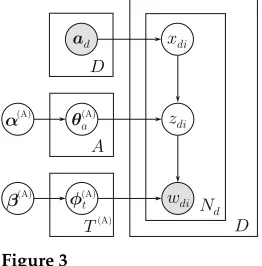
3.3.1 Model Definition.AT was introduced by Rosen-Zvi et al. (2004) to model author interests in corpora of multi-authored texts (e.g., research papers). The main idea behind AT is that each document is generated from the topic distributions of its observed authors, rather than from a document-specific topic distribution. Figure 3 presents AT in plate notation. Formally, the generative process is: (1) for each topict, draw a word distribution φφφ(_tA)∼Dir βββ(A); (2) for each author a, draw a topic

distributionθθθ(aA)∼Dir ααα(A); and (3) for each word indexiin each documentd, draw

an authorxdiuniformly from the document’s set of authorsaaad, a topiczdi ∼Cat θθθ(xAdi)

, and the wordwdi∼Cat φφφ(zAdi)

.

3.3.2 Model Inference.As for LDA, we use collapsed Gibbs sampling to infer AT. This involves repeatedly sampling from Equation (7) (Rosen-Zvi et al. 2004, 2010):

p

xdi=a,

zdi = t

A A

A,WWW,XXX−di,ZZZ−di; ααα(A),βββ(A)

∝ α

(A)

t +c

(AT)

at

PT(A)

t0₌₁

α(_tA0)+c(_atAT0 )

β(wdiA)+c(twATVdi )

PV

v=1

β(vA)+c(tvATV)

(7)

whereXXX−di andZZZ−di are all the author and topic assignments, respectively, excluding

the assignment for the i-th word of the d-th document; c(_atAT) is the count of topic t

assignments to authora; andc_twdi(ATV) is the count of wordwdi in author topic t. Here,

all the counts exclude the di-th assignments (i.e., xdi and zdi). We sample xdi and zdi

w_di D N_d zdi

xdi

D

ad

A

T

Á_t (A) (A) µ_a(A) ®(A)

¯(A)

Figure 3

jointly because this yields faster convergence than separate sampling (Rosen-Zvi et al. 2010).

Similarly to LDA, we estimate the topic and word distributions using their expected values given the author assignmentsXXXand the topic assignmentsZZZ:

E[θ_at(A)|XXX,ZZZ]= α

(A)

t +c

(AT)

at

PT(A)

t0₌₁

α_t(A0)+c(_atAT0 )

(8)

E[φ_tv(A)|ZZZ]= β

(A)

v +c(tvATV)

PV

v0₌₁

β(_vA0)+c(_tvATV0 )

(9)

where in this case the counts are over the full author and topic assignments.

In the classification phase, we do not know the author ˜a of the test text ˜www˜˜ (we assume that test texts are single-authored). If we did, no sampling would be required to obtain ˜a’s topic distribution because it is already inferred in the training phase (Equa-tion (8)). Hence, we assume that ˜ais a “new,” previously unknown author, and utilize Gibbs sampling to infer this author’s topic distribution ˜θθθ˜˜(A) by repeatedly sampling

from Equation (10) (as for LDA, the word distributions are assumed to be observed and set to their expected values according to Equation (9)):

p z˜i=t|www˜˜˜, ˜zzz˜˜−i;ΦΦΦ(A),ααα(A)∝ α

(A)

t +c˜( AT)

t

PT(A)

t0₌₁

α_t(A0)+c˜(_t0AT)

φ

(A)

twi˜ (10)

where ˜zi is the topic assignment for the i-th word in ˜www˜˜, ˜zzz˜˜−i contains all of ˜www˜˜’s topic

assignments except for thei-th assignment, and ˜c(_tAT)is the count of topictassignments to author ˜a(excluding thei-th assignment). Similarly to LDA, we then set ˜θθ˜θ˜(A) to its

expected value according to Equation (8), wherec(_atAT)is replaced with ˜c(_tAT)over the full assignment vector ˜zzz˜˜.

3.3.3 Author Representations.AT naturally yields author representations in the form of distributions over topics. That is, each author ais represented as a distribution over topics θθθa(A). However, AT is limited because all the documents by the same authors

are generated in an identical manner (Section 3.3.1). To address this limitation, Rosen-Zvi et al. (2010) introduced “fictitious” authors, adding a unique “author” to each document. This allows AT to adapt itself to each document without changing the model specification. Therefore, we consider the two following variants: (1)AT: “Pure” AT, without fictitious authors; and (2) AT-FA: AT, when run with the additional pre-processing step of adding a fictitious author to each document.

3.4 DADT

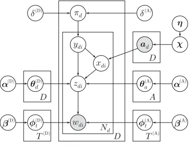
author topics are generated in an AT-like fashion. This approach has the potential ben-efit of separating “document” words from “author” words. That is, words whose use varies across documents are expected to be found in document topics, whereas words whose use varies between authors are expected to be assigned to author topics. Figure 4 presents the graphical representation of the model, where the document-dependent parameters appear on the left-hand side, and the author-dependent parameters appear on the right-hand side. Formally, the generative process is as follows (we mark each step as coming from eitherLDAorAT, or as new inDADT).

Corpus level:

L. For each document topict, draw a word distributionφφφ_t(D)∼Dir βββ(D).

A. For each author topict, draw a word distributionφφφ_t(A)∼Dir βββ(A).

A. For each authora, draw an author topic distributionθθθa(A)∼Dir ααα(A).

D. Draw an author distributionχχχ∼Dir ηηη.

Document level.For each documentd:

L. Drawd’s document topic distributionθθθ_d(D)∼Dir ααα(D).

D. Drawd’s author setaaadby repeatedly sampling without replacement from Cat (χχχ).

D. Drawd’s author/document topic ratioπd ∼Beta δ(A),δ(D).

Word level.For each word indexi∈ {1,. . .,Nd}:

D. Draw the author/document topic indicatorydi ∼Bernoulli(πd).

L. Ifydi=0, use document topics: draw a topiczdi∼Cat θθθ(dD)

, and the wordwdi ∼Cat φφφ(zdiD)

.

A. Ifydi=1, use author topics: Draw an authorxdiuniformly fromaaad,

a topiczdi∼Cat θθθ(xdiA)

, and the wordwdi ∼Cat φφφ(zdiA)

.

It is worth noting that drawing the document’s author set can also be modeled as sampling from Wallenius’s noncentral hypergeometric distribution (Fog 2008) with a weight vectorχχχand a parameter vector whose elements are all equal to 1. In this article,

we consider only situations whereaaad is observed when the model is inferred. When

handling documents with unknown authors in our authorship attribution experiments, we assume that all anonymous texts are single-authored.

(D) (A)

wdi

¯

T D

N_d z_di

Á_t ®

D

µd

y_di

A D

a_d  ´

¼_d ±

(D)

(D) (D)

(D) (D)

±

®(A)

¯(A)

T

Á_t (A) (A) µa

(A)

x_di

Figure 4

3.4.2 Model Inference.We infer DADT using collapsed Gibbs sampling, as done for LDA and AT. This involves repeatedly sampling from the following conditional distribution of the latent parameters:

p

xdi=a,

ydi=y,zdi=t A A

A,WWW,XXX−di,YYY−di,ZZZ−di; ααα(D),βββ(D),δ(D),ααα(A),βββ(A),δ(A)

∝ (11)           

δ(D)+c(_dDD)

_α(D)

t +c

(DT) dt PT(D)

t0=1

α(D)_t0 +c_dt(DT)0

β(D)_wdi+c(DTV)_twdi

PV v=1

β(D)v +c(DTV)tv

ify=0

δ(A)+c(_dDA)

α_t(A)+cat(AT)

PT(A)

t0=1

α(A)

t0 +c

(AT)

at0

β(A)_wdi+c_twdi(ATV)

PV v=1

β(A)v +c(ATV)tv

ify=1

whereYYY−dicontains the topic indicators, excluding thedi-th value; andc_d(DD)andc_d(DA)

are the counts of words assigned to document or author topics in documentd, respec-tively. The other variables are defined as for LDA and AT. Here, all the counts exclude thedi-th assignments (i.e.,xdi,ydi, andzdi).

The building blocks of our DADT model are clearly visible in Equation (11). LDA’s Equation (3) is contained in they=0 case, where the word is drawn from document topics, and AT’s Equation (7) is contained in they=1 case, where the word is drawn from author topics. However, Equation (11) also demonstrates the main difference between DADT and its building blocks, as DADT considersbothdocuments and authors during the inference process by assigning each word to either a document topic or an author topic, where document topics and author topics come from disjoint sets.

As for LDA and AT, we ran several sampling chains in our experiments, retaining samples from each chain after a burn-in period (a sample consists of XXX,YYY, and ZZZ). For each sample, the topic and word distributions are estimated using their expected values given the latent variable assignments. The expected values for the topic and word distributions are the same as for LDA and AT, and the expected values for the author/document ratio and the corpus author distribution are:

E[πd|YYY]=

δ(A)+c(_dDA) δ(D)+δ(A)+Nd

(12)

E[χa|WWW]=

ηa+c(aAD)

PA

a0₌₁

ηa0+c(AD)

a0

(13)

where the counts are now over the full assignmentsXXX,YYY, andZZZ. As in LDA and AT, these equations were straightforward to obtain, because the Dirichlet distribution is the conjugate prior of the categorical distribution and the beta distribution is the conjugate prior of the Bernoulli distribution. It is worth noting that because we assume that the documents’ authors are observed during model inference, the expected value of each element of the corpus distribution over authorsχadoes not vary across samples, as it

only depends on the priorη_aand on authora’s count of documents in the corpusc(aAD).

together with the test text’s document topic distribution ˜θθθ˜˜(D) and author/document

topic ratio ˜πby repeatedly sampling from

p y˜i=y, ˜zi=t|www˜˜˜, ˜yyy˜˜−i, ˜zzz˜˜−i;ΦΦΦ(D),ΦΦΦ(A),ααα(D),ααα(A),δ(D),δ(A)∝ (14) 

    

    

δ(D)+c˜(DD) α (D)

t +c˜(DT)t

PT(D)

t0=1

α(D)_t0 +c˜(DT)_t0

φ

(D)

twi˜ ify=0

δ(A)+c˜(DA) α (A)

t +c˜(AT)t

PT(A)

t0=1

α(A)_t0 +c˜(AT)_t0

φ

(A)

twi˜ ify=1

where ˜yiis the topic indicator for thei-th word, ˜yyy˜˜−icontains all of ˜www˜˜’s topic indicators

except for the i-th indicator, and ˜c(DD) and ˜c(DA) are the counts of words assigned to document and author topics, respectively, excluding thei-th assignment (the other variables are defined as in Equations (6) and (10)). The expected values of ˜θθθ˜˜(D)and ˜θθθ˜˜(A)

are the same as for LDA and AT, respectively. The expected value of ˜π is obtained by

replacingc(_dDA)andNdwith ˜c(DA)and ˜Nin Equation (12) (where ˜c(DA)now contains the

counts over the full vector of indicators ˜yyy˜˜).

3.4.3 Author Representations and Comparison to LDA and AT.DADT can be seen as a gen-eralization of LDA and AT—setting DADT’s number of author topicsT(A)to zero yields a model that is equivalent to LDA, and setting the number of document topicsT(D)to zero yields a model that is equivalent to AT. An advantage of DADT over LDA and AT is that both documents and authors are accounted for in the model’s definition, and are represented via distributions over document and author topics, respectively. Hence, preprocessing steps such as concatenating each author’s documents or adding fictitious authors—as done in LDA-S and AT-FA to obtain author and document representations, respectively—are unnecessary.

Of the LDA and AT variants presented in Sections 3.2.3 and 3.3.3, DADT might seem most similar to AT-FA. However, there are several key differences between DADT and AT-FA.

First, in DADT,author topics are disjoint from document topics, with different priors for each topic set. Thus, the number of author topicsT(A)can be different from the number of document topicsT(D), which enables us to vary the number of author and document topics according to the number of authors and documents in the corpus. For example, in the judgment data set (Section 5.1.1), which includes only a few authors that wrote many long documents, we expect that small values ofT(A) compared to T(D) would suffice to get good author representations. By contrast, modeling the 19,320 authors of the Blog data set (Section 5.1.5) is expected to require many more author topics. On such large data sets, using more than a few hundred topics may become too computationally expensive, because adding topics increases model complexity and thus adds to the runtime of the inference algorithm. Hence, being able to specify the balance between document and author topics in such cases is beneficial (Section 5.4).

Second, DADT places different priors on the word distributionsfor author topics and document topics (βββ(A)andβββ(D), respectively). We know from previous work that

stop-words are strong indicators of authorship (Koppel, Schler, and Argamon 2009). Our model allows us to encode this prior knowledge by giving elements that correspond to stopwords in βββ(A) higher weights than such elements in βββ(D). We found that this

Third, DADT learns the ratio between document words and author words on a per-document basis, and makes it possible to specify a prior belief of what this ratio should be. We show that this has practical benefits in our authorship attribution experiments (Section 5): Specifying a prior belief that on average about 80% of each document is composed of author words can yield better results than using AT’s fic-titious author approach that evenly splits each document into author and document words.

Fourth, DADTdefines the process that generates authors. This allows us to consider the number of texts by each author when performing authorship attribution. In addition, this enables the use of DADT in a semi-supervised setup by training on documents with unknown authors—an extension that is left for future work.

4. Authorship Attribution Methods

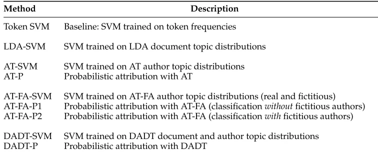
This section introduces the authorship attribution methods considered in this article. In Section 4.1, we discuss our baseline method (SVM trained on tokens), and Sections 4.2, 4.3, 4.4, and 4.5 introduce methods based on LDA, AT, AT-FA, and DADT, respectively. These methods are summarized in Table 2.

We consider two approaches to using topic models in authorship attribution: dimensionality reduction and probabilistic.

Under the dimensionality reduction approach, the original documents are con-verted to topic distributions, and the topic distributions are used as input to a classifier. Generally, this approach makes it possible to use classifiers that are too computationally expensive to use with a large feature set, e.g., Webb, Boughton and Wang’s (2005) AODE classifier, whose time complexity is quadratic in the number of features. We use the reduced document representations as input to SVM, and compare their performance with the performance obtained with SVM trained directly on tokens (denoted Token SVM). This allows us to roughly gauge how much information is lost by converting texts from token representations to topic representations. However, this approach ignores the probabilistic nature of the underlying topic model, and thus does not fully test the utility of the author representations yielded by the model—these are better tested by the next approach.

Table 2

Summary of authorship attribution methods.

Method Description

Token SVM Baseline: SVM trained on token frequencies

LDA-SVM SVM trained on LDA document topic distributions

AT-SVM SVM trained on AT author topic distributions AT-P Probabilistic attribution with AT

AT-FA-SVM SVM trained on AT-FA author topic distributions (real and fictitious) AT-FA-P1 Probabilistic attribution with AT-FA (classificationwithoutfictitious authors) AT-FA-P2 Probabilistic attribution with AT-FA (classificationwithfictitious authors)

In contrast to dimensionality reduction methods,probabilisticmethods utilize the underlying model’s definitions directly to estimate the probability that a given author wrote a given test text. These methods require the model to be aware of authors, which means that LDA cannot be used in this case. We expect this approach to outperform the dimensionality reduction approach because the probabilistic approach considers the structure of the topic model.

An alternative approach that we considered uses a distance measure (e.g., Hellinger distance) to find the author whose topic distributions are closest to the distributions inferred from the test text. We do not describe distance-based methods in this article because we found that they yield poor results in most cases (Seroussi 2012), probably because they do not fully consider the underlying structure of the topic model.

4.1 Baseline: Token SVM

Our baseline method is SVM trained on token frequency features (i.e., token counts divided by the total number of tokens in the document). This method is known to yield state-of-the-art authorship attribution performance on this feature set; that is, when comparing methods without any further feature engineering, Token SVM is expected to yield good performance with minimal tuning (Koppel, Schler, and Argamon 2009). We use the one-versus-all setup to handle non-binary authorship attribution scenarios. This setup scales linearly in the number of authors and was shown to be at least as effective as other multi-class SVM approaches in many cases (Rifkin and Klautau 2004). It is worth noting that unlike the topic models, the Token SVM baseline is trained with the goal of maximizing the authorship attribution accuracy, which may give Token SVM an advantage over topic-based methods. Further, as a discriminative classification approach, SVM may yield better performance than probabilistic topic-based methods, which are generative classifiers (Ng and Jordan 2001). However, as demonstrated by Ng and Jordan’s comparison of discriminative and generative classifiers, this better performance may only be obtained in the presence of “enough” training data (just how much data is “enough” depends on the data set).

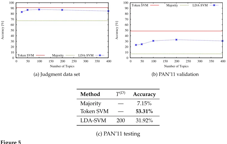
4.2 Methods Based on LDA

4.2.1 Dimensionality Reduction: LDA-SVM.Using LDA for dimensionality reduction is relatively straightforward—all it entails is converting the training and test texts to topic distributions as described in Section 3.2.2, and using these topic distributions as classifier features. Because we use SVM, it is possible to directly compare the results obtained with the LDA-SVM method to the baseline results obtained by running SVM trained directly on token frequencies.

This LDA-SVM approach was utilized by Blei, Ng, and Jordan (2003) to demonstrate the dimensionality reduction capabilities of LDA on the task of classifying articles according to a set of predefined categories. To the best of our knowledge, only Rajkumar et al. (2009) have previously applied LDA-SVM to authorship attribution—they pub-lished preliminary results obtained by running LDA-SVM, but did not compare their results to a Token SVM baseline. In Section 5, we present the results of more extensive experiments on the applicability of this approach to authorship attribution.

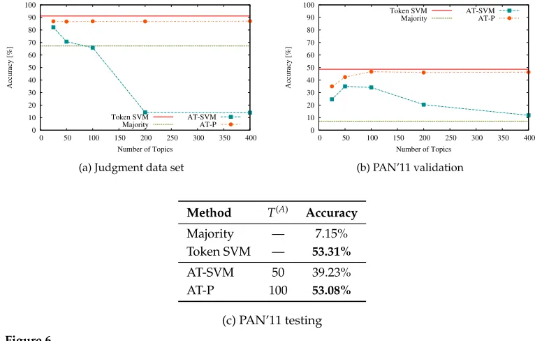
4.3 Methods Based on AT

converted to its author topic distribution). For each test text, we assume that it was written by a previously unknown author, infer this author’s topic distribution ˜θθθ(A)

(Sec-tion 3.3.2), and classify this distribu(Sec-tion. This may be seen as very radical dimensionality reduction, because each author’s entire set of training documents is reduced to a single author topic distribution.

4.3.2 Probabilistic: AT-P.For each authora, AT-P calculates the probability of the test text words given the AT model inferred from the training texts, under the assumption that the test text was written by a. It returns the author for whom this probability is the highest:

arg max

a∈{1,...,A}

p www˜˜˜|a˜=a,ΘΘΘ(A),ΦΦΦ(A)∝ arg max a∈{1,...,A}

˜

N Y

i=1

T(A) X

t=1

θ_at(A)φ(_twiA_˜) (15)

This method does not require any topic inference in the classification phase, because the author topic distributionsΘΘΘ(A)and topic word distributionsΦΦΦ(A)are already inferred at

training time. It is worth noting that we use the log of this probability for reasons of numerical stability.

As mentioned at the beginning of this section, we expect AT-P to outperform AT-SVM because AT-P relies directly on the probabilistic structure of the AT model. In addition, AT-P has the advantage of not requiring any topic inference in the classifi-cation phase.

We also performed preliminary experiments with a method that: (1) assumes that the test text was co-written by all the candidate authors, (2) infers the word-to-author assignments for the test text, and (3) returns the author that was attributed the most words. However, we found that this method performs poorly in comparison with other AT-based approaches in three-way authorship attribution. In addition, this method was too computationally expensive to run in cases with many authors, as it requires iterating through all the authors for every test text word in each sampling iteration.

4.4 Methods Based on AT-FA

AT-FA is the same model as AT, but it is run with the preprocessing step of adding an additional fictitious author to each training document. Hence, different constraints apply to AT-FA in the classification phase. This is because in this phase, we cannot conserve AT-FA’s assumption that all the texts are written by a real author together with a fictitious author, since we do not know who wrote the test text. Hence, if we were to assume that the real author is a previously unknown author, as done for AT, we would have no way of telling the previously unknown author from the fictitious author, because they are both unique to the test text. We consider two possible ways of addressing this:

1. Assume that the test text was written only by a real, previously unknown, author (without a fictitious author), and infer this author’s topic distribu-tion ˜θθ˜θ˜(A)(as in AT).

2. For each training authora, assume that the test text was written byatogether with a fictitious authorfaand infer the fictitious author’s topic distribution ˜θθθ˜˜_fa(A). This

Although the second alternative may appear more attractive because it does not violate the fictitious author assumption of AT-FA, we cannot use it with the dimensionality reduction method (AT-FA-SVM, as described in the following section), as this method requires inferring the topic distribution of the previously unknown author ˜θθθ˜˜(A).

4.4.1 Dimensionality Reduction: AT-FA-SVM.AT-FA yields a topic distribution for each training document (i.e., the topic distribution of the fictitious author associated with the document), and a topic distribution for each real author (all the distributions are over the same topic set). We convert each training document to the concatenation of these two distributions, and use this concatenation as input to the SVM component. In the classification phase, we assume that the test text was written by a single previously unknown author, and represent the test text as the concatenation of the inferred topic distribution ˜θθ˜θ˜(A)to itself.

It is worth noting that our DADT model offers a more elegant solution than con-catenating the same distribution to itself, because DADT differentiates between author topics and document topics—a distinction that AT-FA attempts to capture through fictitious authors. Hence, we expect the DADT-SVM approach, which we define in Section 4.5, to perform better than AT-FA-SVM. Nonetheless, we also experiment with AT-FA-SVM for the sake of completeness.

4.4.2 Probabilistic: AT-FA-P. For the probabilistic approach, we consider two variants, matching the two alternatives outlined earlier.

1. AT-FA-P1.This variant is identical in the classification phase to AT-P—it returns the author that maximizes the probability of the test text’s words according to Equation (15), assuming that the test text wasnotco-written by a fictitious author. 2. AT-FA-P2.This variant performs the following steps for each authora: (1) assume that the test text was written by aand a fictitious author fa; (2) infer the topic

distribution of the fictitious author ˜θθ˜θ˜(_faA); (3) calculate the probability of the test

text words under the assumption that it was written byaandfa, and given the

inferred ˜θθθ˜˜_fa(A); and (4) return the author for whom the probability of the test text

words is maximized:

arg max

a∈{1,...,A}

pwww˜˜˜|aa˜a˜˜, ˜θθθ˜˜(_faA),ΘΘΘ(A),ΦΦΦ(A)

∝ arg max

a∈{1,...,A}

˜

N Y

i=1

T(A) X

t=1

θ_at(A)φ(_twiA_˜)+θ˜_fat(A)φ_t(_wiA_˜)

(16)

where ˜aa˜a˜={a,fa}is the test text’s set of authors.

The problem with this approach is that it is too computationally expensive to use on data sets with many candidate authors, as it requires running a separate inference procedure for each author. Nonetheless, in cases where AT-FA-P2 can be run, we expect it to perform better than AT-FA-P1 because it does not violate the fictitious author assumption of AT-FA.

4.5 Methods Based on DADT

4.5.1 Dimensionality Reduction: DADT-SVM.DADT yields a document topic distribu-tionθθθ(_dD)for each documentd, and an author topic distributionθθθ(aA) for each authora.

In contrast to AT-FA, DADT’s document topic distributions are defined over a topic set that is disjoint from the author topic set. This makes it possible to assume that the test text was written by a previously unknown author, and obtain the test text’s document distribution ˜θθ˜θ˜(D)together with the previously unknown author’s topic

distribution ˜θθ˜θ˜(A)(following the procedure described in Section 3.4.2). As in the training

phase, test texts are represented as the concatenation of these two distributions.

We expect DADT-SVM to outperform AT-FA-SVM, because we are able to main-tain the assumptions of DADT in the classification phase, which we cannot do in AT-FA-SVM. Further, SVM should perform better than AT-SVM, because DADT-SVM accounts for differences between individual documents, whereas AT-DADT-SVM repre-sents each author using a single training instance. Hypothesizing about the expected performance of DADT-SVM in comparison to LDA-SVM is harder: We expect per-formance to be corpus-dependent to a certain degree—in data sets where differences between individual documents are important, LDA-SVM may have an advantage, as all the words are allocated to document topics. On the other hand, in data sets where the differences between authors are more important, DADT-SVM may outperform LDA-SVM because it represents the authors explicitly.

4.5.2 Probabilistic: DADT-P. This method assumes that the test text was written by a previously unknown author, infers the test text’s document topic distribution ˜θθθ˜˜(D)and

the author/document topic ratio ˜π, and returns the most probable author according to

the following equation:

arg max

a∈{1,...,A}

pa˜=a|www˜˜˜, ˜π, ˜θθθ˜˜(D),θθθ(aA),ΦΦΦ(D),ΦΦΦ(A),χa

∝ (17)

arg max

a∈{1,...,A} χa

˜

N Y

i=1



π˜ T(A) X

t=1

θ_at(A)φ_t(A_wi˜)+(1−π˜) T(D) X

t=1 ˜

θ_t(D)φ_t(D_wi˜) 



It is worth noting that in preliminary experiments, we found that an alternative approach that avoids sampling ˜π and ˜θθ˜θ˜(D)by setting ˜π=1 yields poor performance,

probably because it “forces” all the words to be author words, including words that are very likely to be document words. In addition, we found that following an approach where ˜πand ˜θθθ˜˜(D)are sampled separately for each author (similarly to AT-FA-P2) yields

comparable performance to sampling only once by following the previously-unknown author assumption. However, the former approach is too computationally expensive to run on data sets with many candidate authors. Hence, we present only the results obtained with the approach that performs sampling only once.

5. Evaluation

5.1 Data Sets

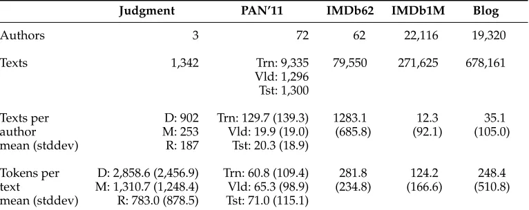
We experimented with five data sets: Judgment, PAN’11, IMDb62, IMDb1M, and Blog. Judgment, IMDb62, and IMDb1M were collected and introduced by us, and are freely available for research use (Judgment can be downloaded from www.csse. monash.edu.au/research/umnl/data, and IMDb62 and IMDb1M are available upon request). The two other data sets were introduced by other researchers, are publicly available, and were used to facilitate comparison between our methods and previous work. Table 3 presents some data set statistics.

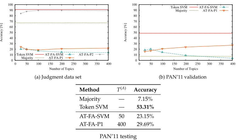
5.1.1 Judgment.The Judgment data set contains judgments by three judges who served on the Australian High Court from 1913 to 1975: Dixon, McTiernan, and Rich (ab-breviated to D, M, and R, respectively, in Table 3). We created this data set to verify rumors that Dixon ghost-wrote some of the judgments attributed to McTiernan and Rich (Seroussi, Smyth, and Zukerman 2011). This data set is an example of a traditional authorship attribution data set, as it contains only three authors who wrote relatively long texts in a formal language. In this article, we only use judgments with undisputed authorship, which were written in periods when only one of the three judges served on the High Court (Dixon’s 1929–1964 judgments, McTiernan’s 1965–1975 judgments, and Rich’s 1913–1928 judgments). We removed numbers from the texts to ensure that dates cannot be used to discriminate between judges. We also removed quotes to ensure that the classifiers take into account only the actual authors’ language use (removal was done automatically by matching regular expressions for numbers and text in quotation marks). Because all three judges dealt with various topics, it is likely that successful methods would have to consider each author’s style, rather than rely solely on content features in the texts.

As Table 3 shows, the Judgment data set contains the smallest number of authors of the data sets we considered, but these authors wrote more texts than the average author in PAN’11, IMDb1M, and Blog. Judgments are also substantially longer than the texts in all the other data sets, which should make authorship attribution on the Judgment data set relatively easy.

Table 3

Data set statistics.

Judgment PAN’11 IMDb62 IMDb1M Blog

Authors 3 72 62 22,116 19,320

Texts 1,342 Trn: 9,335 79,550 271,625 678,161

Vld: 1,296 Tst: 1,300

Texts per D: 902 Trn: 129.7 (139.3) 1283.1 12.3 35.1 author M: 253 Vld: 19.9 (19.0) (685.8) (92.1) (105.0) mean (stddev) R: 187 Tst: 20.3 (18.9)

5.1.2 PAN’11. The PAN’11 data sets were introduced as part of the PAN 2011 compe-tition (available frompan.webis.de) (Argamon and Juola 2011). These data sets were extracted from the Enron e-mail corpus (www.cs.cmu.edu/~enron), and were designed to emulate closed-class and open-class authorship attribution and authorship verifica-tion scenarios (Secverifica-tion 2). These data sets represent authorship attribuverifica-tion scenarios that may arise in computer forensics, such as the case noted by Chaski (2005), where an employee who was terminated for sending a racist e-mail claimed that any person with access to his computer could have sent the e-mail.

In our experiments, we used the largest PAN’11 data set, with e-mails by 72 authors. Unlike the other data sets we used, this data set is split into training, validation, and testing subsets (abbreviated to Trn, Vld, and Tst, respectively, in Table 3). We focused on the closed-class problem, using the validation and testing sets that contain texts only by training authors. The only change we made to the original data set was dropping two training and two validation texts that were automatically generated, which were detected by length and content. This had a negligible effect on method accuracy, but made the statistics in Table 3 more representative of the data (e.g., the mean count of tokens per text is 65.3 in the validation set without the two automatically generated texts, compared with 338.3 in the full validation set).

Using this data set allows us to test our methods on short and informal texts with more authors than in traditional authorship attribution. As Table 3 shows, the PAN’11 data set contains the shortest texts of the data sets we considered. This fact, together with the training/validation/testing structure of the data set, make it possible to run many experiments on this data set before moving on to larger data sets.

5.1.3 IMDb62.IMDb62 contains 62,000 movie reviews and 17,550 message board posts by 62 prolific users of the Internet Movie database (IMDb, www.imdb.com). We intro-duced this data set (Seroussi, Zukerman, and Bohnert 2010) to test our author-aware polarity inference approach (Section 6.2). Each user wrote 1,000 reviews (sampled from their full set of reviews), and a variable number of message board posts, which are mostly movie-related, but may also be about television, music, and other topics. This data set allows us to test our approach in a setting where all the texts have similar themes, and the number of authors is relatively small, but is already much larger than the number of authors considered in traditional authorship attribution settings. Unlike the other data sets of informal texts, IMDb62 consists only of prolific authors, allowing us to test our approach in a scenario where training data is plentiful.

5.1.4 IMDb1M.Although the IMDb62 data set is useful for testing our methods on small-to medium-scale problems, it cannot be seen as an adequate representation of large-scale problems. This is especially relevant to the task of rating prediction, in which typical data sets contain thousands of users (Section 6.3). Hence, we created IMDb1M by randomly generating one million valid IMDb user IDs and downloading the reviews and message board posts written by these users (Seroussi, Bohnert, and Zukerman 2011). Unfortunately, most of the randomly generated IDs led to users who submit-ted neither reviews nor posts—we found that about 5% of the entire user population submitted posts, and less than 3% wrote reviews. After filtering out users who have not submitted any rated reviews, we were left with 22,116 users. These users, who make up the IMDb1M data set, submitted 204,809 posts and 66,816 rated reviews.

IMDb1M contains a more varied sample of the population. However, because we did not impose a minimum threshold on the number of reviews or posts, the IMDb1M population is very challenging as it includes many users with few texts (e.g., about 56% of the users in IMDb1M wrote only one text). It is worth noting that three users appear in both IMDb62 and IMDb1M. In IMDb62 these three users authored 3,000 reviews and 268 posts in total (about 4.8% of the total number of reviews and 1.5% of the posts), and in IMDb1M they authored 5,695 reviews and 358 posts (about 8.5% of the re-views and 0.2% of the posts). The difference in the number of rere-views is due to the sampling we performed when we created IMDb62, and the difference in the number of posts is due to the time difference between the creation of the two data sets.

5.1.5 Blog. The Blog data set is the largest data set we consider, containing 678,161 blog posts by 19,320 authors (available fromu.cs.biu.ac.il/~koppel). It was created by Schler et al. (2006) to learn about the relation between language use and demographic characteristics, such as age and gender. We use this data set to test how our authorship attribution methods scale to handle thousands of authors. As blog posts can be about any topic, this data set is less restricted than the Judgment, PAN’11, and IMDb data sets. Further, the large number of authors ensures that every topic is likely to interest at least several authors, meaning that methods that rely only on content are unlikely to perform as well as methods that also take author style into account.

5.2 Experimental Setup

We used different experimental setups, depending on the data set. PAN’11 experiments followed the setup of the PAN’11 competition (Argamon and Juola 2011): We trained all the methods on the given training data set, tuned the parameters according to results obtained for the given validation data set, and ran the tuned methods on the given testing data set. For all the other data sets we utilized ten-fold cross validation. In all cases, we report the overall classification accuracy, that is, the percentage of test texts correctly attributed to their author. Statistically significant differences are reported when p<0.05 according to McNemar’s test (when reporting results in a table, the best result for each column is in boldface, and several boldface results mean that the differences between them are not statistically significant).

In our experiments, we used the L2-regularized linear SVM implementation of LIBLINEAR (Fan et al. 2008), which is well suited for large-scale text classification. We experimented with cost parameter values from the set{. . ., 10−1, 100, 101,. . .}, until no accuracy improvement was obtained (starting from 100=1 and going in both direc-tions). We report the results obtained with the value that yielded the highest accuracy, which gives an optimistic estimate for the performance of the Token SVM baseline.