Applying Computational Models of Spatial Prepositions to Visually Situated Dialog

Prepositions to Visually Situated Dialog

John D. Kelleher

Dublin Institute of Technology

Fintan J. Costello

This article describes the application of computational models of spatial prepositions to visually situated dialog systems. In these dialogs, spatial prepositions are important because people often use them to refer to entities in the visual context of a dialog. We first describe a generic architecture for a visually situated dialog system and highlight the interactions between the spatial cognition module, which provides the interface to the models of prepositional semantics, and the other components in the architecture. Following this, we present two new computational models of topological and projective spatial prepositions. The main novelty within these models is the fact that they account for the contextual effect which other distractor objects in a visual scene can have on the region described by a given preposition. We next present psycholinguistic tests evaluating our approach to distractor interference on prepositional semantics, and illustrate how these models are used for both interpretation and generation of prepositional expressions.

1. Introduction

A growing number of computer applications share a visualized(virtual or real) space with the user, for example graphic design programs, computer games, navigation aids, robot systems, andso forth. If these systems are to be equippedwith dialog interfaces, they must be able to participate in visually situateddialog. Visually situateddialog is spoken from a particular point of view within a physical or simulatedcontext. From theoretical linguistic andcognitive perspectives, visually situateddialog systems are interesting as they provide ideal testbeds for investigating the interaction between language andvision. From a human–computer interaction (HCI) perspective, visually situated dialog systems promise many advantages to users interacting with these systems. In this article we describe computational models for the interpretation and generation of visually situatedlocative expressions involving topological andprojective spatial prepositions.

ContributionsAn inherent aspect of visually situateddialog is reference to objects in the physical environment in which the dialog occurs. People often use locative

∗School of Computing, Dublin Institute of Technology, Kevin Street, Dublin 8, Ireland. E-mail: [email protected].

∗∗School of Computer Science and Informatics, University College Dublin, Belfield, Dublin 4, Ireland. E-mail: fi[email protected].

expressions, in particular spatial prepositions, to pick out objects in the visual envi-ronment. In this article we present computational models of the semantics of spatial prepositions andillustrate how these models can be usedin a visually situateddialog system for reference resolution and generation. These models are designed to handle reference resolution andgeneration in complex visual environments containing multi-ple objects, andto account for the contextual influence which the presence of multimulti-ple objects has on the semantics of spatial prepositions. In this our models move beyond other accounts, which typically do not model the contextual influence of other objects on spatial semantics. Because most real-worldvisual scenes are complex andcontain multiple objects, our models for the semantics of spatial prepositions are important for visually situated dialog systems intended to operate usefully in the real world.

Overview We begin in Section 2 by describing some terminology we use when discussing locative expressions. In Section 3 we present an abstract architecture for a visually situated dialog system and, using this architecture, illustrate how the spa-tial reasoning component of the architecture interacts with the other components of the system. In Section 4 we review psycholinguistic data on the semantics of spatial prepositions. Section 5 reviews previous computational models of spatial prepositional semantics. Section 6 presents our computational models accounting for the semantics of spatial prepositions andthe influence of visual context on those semantics, andSection 7 presents psycholinguistic evaluation of these models. Section 8 presents applications of the models in implemented systems. Section 8.1 presents an application of our models to the interpretation of locative expressions, basedon Kelleher, Kruijff, andCostello (2006), andSection 8.2 presents algorithms which use these models to generate locative expressions to identify objects in visual scenes from Kelleher and Kruijff (2006).

2. Terminology

Our computational models are designed to interpret and generatelocative expressions involving spatial prepositions. The term locative expression describes “an expression involving a locative prepositional phrase together with whatever the phrase modifies (noun, clause, etc.)” (Herskovits 1986, page 7). In this article we use the term target (T) to refer to the object that is being locatedby a locative expression andthe term landmark1(L) to refer to the object relative to which the target’s location is described; see Example (1). We will use the termdistractor to describe any object in the visual context that is neither the landmark nor the target.

Example 1

[The man]T near [the table]L.

The English lexicon of spatial prepositions numbers above 80 members (not consid-ering compounds such asright next to) (Landau 1996). Within this set a distinction can be made between static and dynamic prepositions: static prepositions primarily2denote

1 There is a wealth of terms usedin the literature describing locative expressions. The termslocal object,

figure object, andtrajectorare all equivalent to our termtargetwhile the termsreference object,ground, andrelatumare equivalent to our termlandmark.

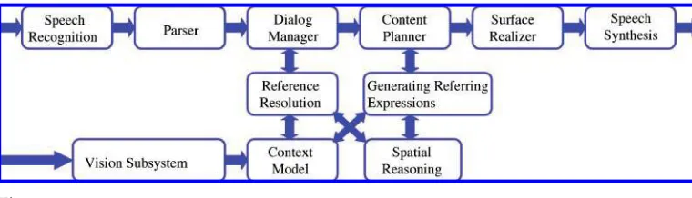
Figure 1

Architecture of a visually situateddialog system.

the location of an object, dynamic prepositions primarily denote the path of an object (Jackendoff 1983; Herskovits 1986), see Examples (2) and (3).

Example 2

The tree is [behind]static the house.

Example 3

The man walked[across]dynamic the road.

In general, the set of static prepositions can be decomposed into two sets called topological and projective. Topological prepositions are the category of prepositions referring to a region that is proximal to the landmark; for example,at,near. Often, the distinctions between the semantics of the different topological prepositions is based on pragmatic constraints, for example the use ofatlicenses the target to be in contact with the landmark, while the use ofneardoes not. Projective prepositions describe a region projected from the landmark in a particular direction, with the specification of the direction dependent on theframe of reference3being used; for example,to the right of,to the left of.

3. Visually Situated Dialog System Architecture

In this section we present an abstract implementation-independent architecture for a visually situateddialog system andhighlight the role playedby spatial reasoning in the functioning of the system. In particular, we describe how models of spatial prepositional semantics are important for reference resolution andgeneration.

The distinguishing characteristic of a visually situated dialog system is that the system has the ability to visually perceive the environment in which a dialog is situated. Consequently, these systems use both visual andlinguistic contextual information to understand user commands and to generate linguistic descriptions of the environment. Figure 1 illustrates the visual dialog system architecture we will describe. The arrows in the figure represent data flows through the system; the boxes are the main information processing components.

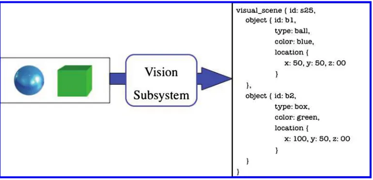
Figure 2

Example input andoutput data from a vision subsystem.

There are two information inputs into this system: the vision subsystem andthe speech interpretation pipeline. The vision subsystem directly updates the system’s representation of the visual context. The basic requirements for the vision subsystem are that it is able to detect andcategorize the objects in the visual context andcan provide geometric positioning information for each visible object. Figure 2 illustrates the analysis that a vision subsystem may generate for a given scene.

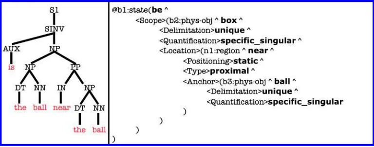
The speech interpretation pipeline begins with speech recognition. This module takes a speech utterance from the user andcreates a string representation of it. The parser uses this string to construct a structuredrepresentation of the input. Parsers range in function from wide-coverage syntactic focused parsers, such as Cahill et al.’s (2004) probabilistic Lexical-Functional Grammar (LFG) parser, to narrow coverage se-mantic basedparsers, for example the CoSy parser (Kruijff, Kelleher, andHawes 2006). Figure 3 illustrates the types of analyses produced by these different types of parsers for the input stringis the box near the ball? The parse tree on the left was generatedusing a probabilistic wide-coverage LFG parser.4The parse tree provides a syntactic analysis of the input string.

Generally, parsers developed for interactive dialog systems integrate semantic, as well as syntactic, information in their grammars. In these parsers the elements in the lexicon andgrammar are basedon an analysis of the entities andrelations of the specific domain the system is designed for. These parsers sacrifice coverage for depth of analysis. For a dialog system, the advantage of this deeper analysis is that the semantic information in the parser’s output can be usedby the dialog manager to relate the input to the rest of the dialog. The parse structure on the right of Figure 3 illustrates the type of semantically rich representation that an interactive dialog system parser might produce (this particular representation was generatedby the CoSy parser).

The CoSy parser uses a Combinatory Categorial Grammar that represents linguistic meaning using an ontologically rich sorted relational structure (Baldridge and Kruijff

Figure 3

Example parse structures for the stringis the box near the ball?

2002, 2003). Within this representation the statementb2:phys-objmeans that the referent b2 is of type phys-obj (i.e., a physical object as defined by the ontology the grammar in-dexes). The semantic contribution of the prepositional phrasenear the ballis represented by the<Location>structure andits subcomponents. This structure describes a locative prepositional phrase containing a static preposition that locates the referent b2 in the regionrthat is proximal to the landmark described by the<Anchor>subcomponent. It shouldbe notedthat the syntactic andsemantic representation of prepositions within grammars is an area of ongoing research (see Gawron 1986; Tseng 2000; Beermann and Hellan 2004). The analysis presentedhere of the prepositional phrase near the ball is intended to illustrate some of the semantic features that prepositions may introduce into a grammar andis not intendedas a comprehensive account of how prepositions shouldbe grammatically represented.

The final stage in the interpretation pipeline is to categorize how the utterance relates to the current dialog context. This categorization is driven by the dialog manager andinvolves interpreting an utterance as a dialog act(Bunt 1994; Carletta et al. 1997; Klein 1999). One of the important tasks in this process is resolving the references in the input. Consequently, the dialog manager may invoke the reference resolution component. Reference resolution is one of two functions in the architecture where spatial reasoning plays an important role. From a computational perspective, reference resolution involves two main tasks:

1. Creating and maintaining a model of what the system considers as mutual knowledge (this model should contain all the objects that are available for reference andtheir properties)

2. Matching the representation introduced by a given referring expression to an element (or elements) in the set of possible referents

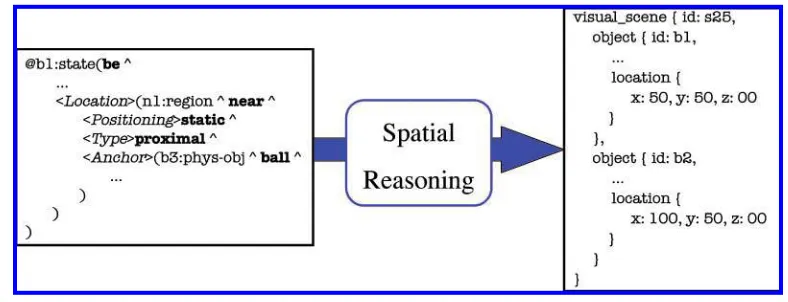
Figure 4

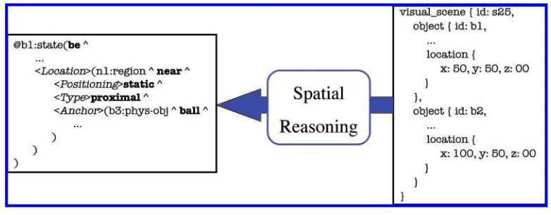
The mapping performedby the spatial reasoning module from qualitative to geometric representations during the interpretation of a locative expression.

used. In this architecture this access is provided through the spatial reasoning compo-nent. Figure 4 illustrates the translation between the qualitative, parser-generated, and the geometric, vision subsystem–generatedrepresentations that must be performedin order to interpret a spatial locative expression.

At different stages during a dialog the dialog manager may recognize that the system needs to generate a response to the last input utterance. For example, the utterance may have been a question, such as where is x? or which x?. In such cases, the dialog manager informs the content planner of this. The role of the content planner is to determine the semantic content that should be included in the system’s output, rather than the linguistic realization of this content. Indeed, the content planner may generate a logical representation closer to the parse structure on the right of Figure 3 than to a natural language description.

Generating referring expressions (GRE) is a key stage in content planning. GRE is the secondfunction in the architecture where spatial reasoning plays an important role. The function of the GRE component is to determine the set of properties that distinguish a particular target object from the other objects in the scene. For example, in response to a question such aswhich x?the GRE component may determine that a color and type description is sufficient to distinguish the target object, resulting in an answer such asthe blue xbeing linguistically realized. However, it may be the case that the location of the target in the scene is the only way to distinguish it. In such cases, the GRE component needs access to computational models of the spatial prepositions if it is to determine which spatial relation is most suitable. Figure 5 illustrates the translation from a geo-metric to qualitative representation that is performedduring the GRE process by the spatial reasoning module when a locative description is being generated by the system. Once the content planning andGRE processes have been completed, the realizer determines a surface linguistic form in which this content can be conveyed. Finally, the speech synthesis systems generate the speech output for the linguistic string createdby the realizer.

4. Psycholinguistic Data on Spatial Prepositions

Figure 5

The mapping performedby the spatial reasoning module from geometric to qualitative to representations during the generation of a locative description.

(Herskovits 1986), andafunctional levelwhere the normal function of an entity affects the spatial relationships attributedto it in a context (Coventry andGarrod2004).

There has been much experimental work done on spatial reasoning and language. Some of this work has focusedon functional aspects of prepositional semantics (e.g., HaywardandTarr 1995; Coventry 1998; Garrod, Ferrier, andCampbell 1999), andsome on geometric factors (Gapp 1995; Logan andSadler 1996; Regier andCarlson 2001). In this article we are primarily concernedwith the geometric semantics of prepositions and, consequently, our review will focus on the experimental data that addresses geo-metric factors. We will begin by reviewing the experimental data describing topological spatial prepositions. Following this, we will then review data relating to projective prepositions.

Topological prepositions denote a region that is proximal to a landmark. Subse-quently we discuss previous psycholinguistic experiments, focusing on how contex-tual factors such as distance, size, and salience may affect proximity. We also present examples showing that the location of other objects in a scene may interfere with the acceptability of a proximal description to locate a target relative to a landmark.

Logan andSadler (1996) examinedthe semantics of several spatial prepositions. In their experiments, a human subject was shown sentences of the formthe X is [relation] the O, each with a picture of a spatial configuration of anOin the center of an invisible 7 ×7 cell grid, and anXin one of the 48 surrounding positions. The subject then had to rate how well the sentence described the picture, on a scale from 1 (bad) to 9 (good). Figure 6 gives the mean goodness rating for the relation “near to” as a function of the position occupiedby X (Logan andSadler 1996). It is clear from Figure 6 that ratings diminish as the distance between X and O increases, but also that even at the extremes of the gridthe ratings were still above 1 (minimum rating).

Besides distance there are also other factors that determine the applicability of a proximal relation. For example, given prototypical size, the region denoted bynear the buildingis larger than that ofnear the apple. Moreover, an object’s salience couldinfluence the determination of the proximal region associated with it; as with size, the more salient an object is the larger the proximal region associatedwith it (Gapp 1994).

Figure 6

A 7×7 cell grid with mean goodness ratings for the relationthe X is near Oas a function of the position occupiedby X.

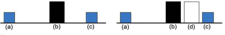
to interfere with the appropriateness of using a proximal relation to locate (c) relative to (b), even though the absolute distance between (c) and (b) has not changed.

There are several important features that are evident from these data. First, given a context, subjects have the ability to grade the applicability of a spatial relation. Logan and Sadler (1996) introduced the termspatial templateto describe the representation of the regions of acceptability associatedwith a preposition. A spatial template is centered on the landmark and identifies for each point in its space the acceptability of the spatial relationship between the landmark and the target appearing at that point being described by the preposition. Second, there is empirical evidence pointing to the effects of distance between that landmark and the target, and landmark salience and size on the applicability of a proximity-basedpreposition. Finally, the examples presentedpoint to the fact that the location of other distractor objects in context may also interfere with the applicability of a preposition. (The model of proximity we present in Section 6 captures all these factors.)

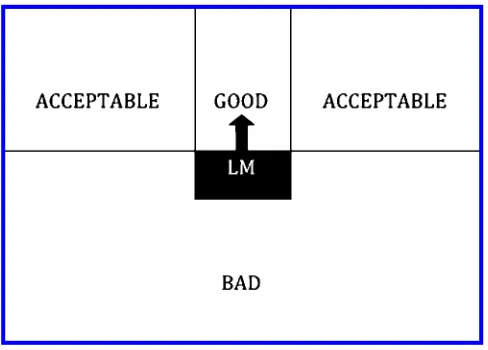
Figure 8 is a representation of the spatial template for the projective preposition

above described in Logan and Sadler (1996). The main points of note relating to these data are that there are three regions in the spatial template (good, acceptable, and bad) and these regions are symmetric around the canonical direction of the preposition with acceptability approaching 0 as the angular deviation from the canonical direction approaches 90 degrees. However, it should be noted that these data were gathered dur-ing an interpretation task andthat the task may have affectedthe subjects’ responses.

Figure 7

Figure 8

Spatial template for the prepositionabove(Logan andSadler 1996), where LM represents the landmark and the arrow shows the canonical direction associated with the preposition.

Although the subjects may have ratedsome of the areas on the far right andleft of the landmark as acceptable with respect to interpreting an utterance such as above the landmark, this does not mean that they would use the wordaboveto describe a target object in these regions relative to the landmark. This highlights the fact that people may be more accommodating when they are interpreting a locative description (for example, they may extend the allowable angular deviation to 90 degrees) but be more specific when generating a locative description.

5. Previous Models of Topological and Projective Spatial Prepositions

There has been much research on the formal properties andinteractions of topological relations, for example Cohn et al. (1997) andKuipers (2000). However, before these higher-level frameworks can be applied to real-world data, a model of proximity that is capable of segmenting a region at the metric or geometric level is required. At this geometric level previous approaches to modeling topological prepositions have adopted one of two approaches to defining the region of proximity. The first is to adopt a Voronoi segmentation of space. Under this approach the region considered as proximal to an object is the area surrounding it that is closer to it than to any other object in the scene. The second is to define the proximal region in terms of the size of the landmark. For example, Gapp (1995) defines the area of proximity as the region within ten times the size of the landmark object in each direction. However, neither of these approaches consider the effect that the locations of other objects in the scene have on the proximity. Consequently, they cannot distinguish between the different context provided by the two images in Figure 7.

(2006) developed a computational model that constructed a modified spatial template in situations where frame of reference ambiguity occurred. Fuhr et al. (1998) used models of prepositional semantics in order to interpret natural language commands to a robotic arm. Fuhr et al. segmentedthe space aroundan object into different regions based on the sides and vertices of the object’s bounding box. One of the drawbacks of this system, however, was that it couldnot distinguish between the position of two or more objects that were fully enclosedwithin a given region. Finally, Regier andCarlson (2001) developed a vector sum algorithm to compute the applicability of a projective relation between a landmark and a target. However, as with previous topological models, none of these models consider the influence of other objects in the context of the landmark target relationship. For example, the introduction of the long black object into image 2 in Figure 9 affects the interpretability of a reference such asthe blue square above the white rectangle. In the next section we describe new models designed to account for the influence of other objects in the semantics of spatial prepositions.

6. Models of Visual Context in Topological and Projective Spatial Prepositions

If a computational model is going to accommodate the gradation of applicability across a preposition’s spatial template it must define the semantics of the preposition as some sort of continuum function. A potential field modelis one form of continuum measure that is widely used (Yamada 1993; Gapp 1994; Olivier and Tsujii 1994; Regier andCarlson 2001). Using this approach, a model of a preposition’s spatial template is constructedusing a set of normalizedequations that, for a given origin andpoint, computes a value that represents the cost of accepting that point as the interpretation of the preposition.

Each equation usedto construct the potential fieldrepresentation of a preposition’s spatial template models a different geometric constraint specified by the preposition’s semantics. For example, for topological prepositions such asnear, an equation inversely proportional to the distance between a point and a landmark would be used, while for projective prepositions such asto the right of, an equation modeling the angular de-viation of a point from the idealized direction denoted by the preposition would be in-cludedin the construction set; Gapp (1995) andLogan andSadler (1996) both notedthat acceptability of a projective preposition being usedto describe a location approaches 0 as the angular deviation of that location approaches 90 degrees. The potential field is then constructedby assigning each point in the fieldan overall potential by inte-grating the results computedfor that point by each of the equations in the construc-tion set.

Figure 9

This potential fieldapproach does not, however, account for the influence of other objects in the visual scene on the semantics of a topological or projective preposition. The basic idea in our computational models is to extend the potential field approach by overlaying the potential fields for each object in a visual scene and combining those fields to produce relative potential fields for topological or projective prepositions. These relative potential fields represent the semantics of those prepositions as modified by the presence of other objects in the visual scene.

6.1 Computational Model of Topological Prepositions

In this section we describe a model of relative proximity that uses (1) the distance between objects, (2) the size andsalience of the landmark object, and(3) the location of other objects in the scene. Our model is based on first computing absolute proximity between each point andeach landmark in a scene, andthen combining or overlaying the resulting absolute proximity fields to compute the relative proximity of each point to each landmark.

6.1.1 Computing Absolute Proximity Fields. We first compute for each landmark an ab-solute proximity fieldgiving each point’s proximity to that landmark, independent of proximity to any other landmark. We compute fields on the projection of the scene onto the 2D-plane, representedas a 2D-array of points. At each point P in thatarray, the absolute proximity for landmarkLis

proxabs(L,P)=(1−distnormalized(L,P))∗salience(L) (1)

In this equation the absolute proximity for a pointPanda landmarkLis a function of both the distance between the point and the location of the landmark, and the salience of the landmark.

To represent distance we use a normalized distance function distnormalized(L,P),

which returns a value between 0 and1.5 The smaller the distance between Land P, the higher the absolute proximity value returned, that is, the more acceptable it is to say thatPis close toL. In this way, this component of the absolute proximity fieldcaptures the gradual gradation in applicability evident in Logan and Sadler (1996).

We model the influence of visual and discourse salience on absolute proximity as a function salience(L), returning a value between 0 and1 that represents the relative salience of the landmark L in the scene (Equation (2)). For the current purposes we assume that the relative salience of an object is the average of its visual salience (S_vis) anddiscourse salience (S_disc).6

salience(L)=(Svis(L)+Sdisc(L))/2 (2)

5 We normalize by computing the distance between the two points, and then dividing this distance by the maximum distance between pointLandany point in the scene.

Visual salienceSvisis computedusing the algorithm of Kelleher andvan Genabith

(2004). Computing a relative salience for each object in a scene is basedon its perceivable size andits centrality relative to the viewer’s focus of attention. The algorithm returns scores in the range of 0 to 1. As the algorithm captures object size, we can model the effect of landmark size on proximity through the salience component of absolute proximity. The discourse salience (S_disc) of an object is computedbasedon recency of mention (Hajicov ´a 1993) except we represent the maximum overall salience in the scene as 1, and use 0 to indicate that the landmark is not salient in the current context.

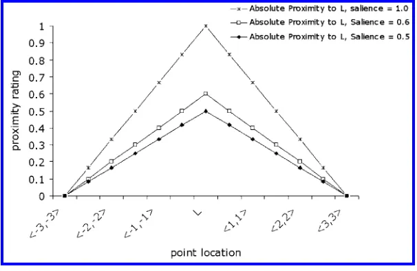
Figure 10 shows computedabsolute proximity with salience values of 1, 0.6, and 0.5, for points from the upper-left to the lower-right of a 2D plane, with the landmark at the center of that plane. The graph shows how salience influences absolute proximity in our model: For a landmark with high salience, points far from the landmark can still have high absolute proximity to it.

6.1.2 Computing Relative Proximity Fields.Once we have constructedabsolute proximity fields for the landmarks in a scene, our next step is to overlay these fields to produce a measure ofrelative proximityto each landmark at each point. For this we first select a landmark, and then iterate over each point in the scene comparing the absolute proximity of the selectedlandmark at that point with the absolute proximity of all other landmarks at that point. The relative proximity of a selected landmark at a point is equal to the absolute proximity fieldfor that landmark at that point, minus the highest absolute proximity fieldfor any other landmark at that point:

proxrel(P,L)=proxabs(P,L)− MAX ∀LX=L

proxabs(P,LX) (3)

The idea here is that the other landmark with the highest absolute proximity is acting in competition with the selected landmark. If that other landmark’s absolute proximity

Figure 10

is higher than the absolute proximity of the selectedlandmark, the selectedlandmark’s

relativeproximity for the point will be negative. If the competing landmark’s absolute proximity is slightly lower than the absolute proximity of the selectedlandmark, the selectedlandmark’srelativeproximity for the point will be positive, but low. Only when the competing landmark’s absolute proximity is significantly lower than the absolute proximity of the selected landmark will the selected landmark have a high relative proximity for the point in question.

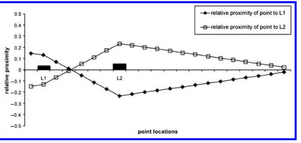
In Equation (3) the proximity of a given point to a selectedlandmark rises as that point’s distance from the landmark decreases (the closer the point is to the land-mark, the higher its proximity score for the landmark will be), butfallsas that point’s distance from some other landmark decreases (the closer the point is to some other landmark, the lower its proximity score for the selected landmark will be). Figure 11 shows the relative proximity fields of two landmarks, L1 and L2, computed using Equation (3) in a 1-dimensional (linear) space. The two landmarks have different de-grees of salience: a salience of 0.5 for L1 andof 0.6 for L2 (representedby the different sizes of the landmarks). In this figure, any point where the relative proximity for one particular landmark is above the zero line represents a point which is proximal to that landmark, rather than to the other landmark. The extent to which that point is above zero represents its degree of proximity to that landmark. The overall proximal area for a given landmark is the overall area for which its relative proximity field is above zero. The left and right borders of the figure represent the boundaries (walls) of the area.

Figure 11 illustrates three main points. First, the overall size of a landmark’s prox-imal area is a function of the landmark’s position relative to the other landmark and to the boundaries. For example, landmark L2 has a large open space between it and the right boundary: Most of this space falls into the proximal area for that landmark. Landmark L1 falls into quite a narrow space between the left boundary and L2. L1 thus has a much smaller proximal area in the figure than L2. Second, the relative proximity field for a landmark is a function of that landmark’s salience. This can be seen in Figure 11 by considering the space between the two landmarks. In that space the width of the proximal area for L2 is greater than that of L1, because L2 is more salient.

Figure 11

Figure 12

Example scene.

The thirdpoint concerns areas of ambiguous proximity in Figure 11: areas in which neither of the landmarks have a significantly higher relative proximity than the other. There are two such areas in the Figure. The first is between the two landmarks, in the region where one relative proximity fieldline crosses the other. These points are ambiguous in terms of relative proximity because these points are equidistant from those two landmarks. The second ambiguous area is at the extreme right of the space shown in Figure 11. This area is ambiguous because this area is distant from both landmarks: Points in this area would not be judged proximal to either landmark. The question of ambiguity in relative proximity judgments is considered in more detail in Section 8.1.

We will illustrate the different stages of the proximity model using the situation illustrated in Figure 12. The task is to decide whether the target object is proximal to the landmark object. Figure 13 illustrates the absolute potential field for the landmark

Figure 13

Figure 14

The absolute proximity fields for the landmark and the distractor.

object. Figure 14 illustrates the absolute potential fields for the landmark and the distractor object. Figure 15 illustrates the relative proximity field that results from the interaction between the landmark and distractors absolute proximity fields. Figure 16 illustrates the application of the threshold to the landmark’s relative proximity field. If the target object is locatedin the region where the landmark’s relative proximity field

Figure 15

Figure 16

Applying the threshold to the landmark’s relative proximity field.

is above the thresholdthe target is deemedto be proximal to the landmark. Figure 16 demonstrates the contextual influence which the distractor object has on the landmark’s relative proximity field: The field shrinks on the side of the landmark near the distractor, but expands on the side away from the landmark.

6.2Computational Model of Projective Prepositions

The two main factors that impact on the applicability of a projective preposition de-scribing the spatial relationship between a target object anda landmark are the angular deviation of the target object’s position from the canonical direction described by the preposition relative to the landmark and the distance of the target object from the landmark.

The vector originating from the center of the landmark to the viewer’s position describes the canonical search axis for in front of. We can produce the search vectors for the other projective prepositions (behind,left,right) by rotating this front vector on a horizontal plane. Once the canonical vectorcfor a given projective preposition has been selected, the angular deviation of a given pointPposition relative to the landmarkLcan be computedusing Equation (4):

angle(LP,c)=cos−1   _LP •_c

_LP |_c|



 (4)

Using this equation, and the normalized distance measure described in Section 6.1, we define an absolute potential field for the acceptability of a projective preposition with canonical vectorcfor land mark L as follows:

projabs(L,P,c)=0if (angle(LP ,c)>90)or(distnormalized(L,P)=0),

=(angle(LP ,c)/dist_normalized(L,P))otherwise (5)

In this equation, if the angle between a pointPandthe canonical vectorcis greater than 90 degrees, or if the distance between the landmark and the point is 0, the acceptability of that point for the projective preposition is 0. Otherwise, the acceptability of that point is equal to the angle between that point and the canonical vector, divided by the normalized distance between that point and the landmark.

We use this absolute potential fieldfor projective prepositions in the same way that we usedthe absolute fieldfor proximity in our model of topological prepositions. Once we have computedthe absolute potential fieldfor each point relative to the landmark we then do the same process for each of the distractor landmarks. We then overlay the landmark applicabilities with those of the distractors by subtracting the maximum applicability of any of the distractors at a point from the landmark’s applicability at that point, producing a relative potential field for the projective prepo-sition as in Equation (6):

projrel(P,L,c)=projabs(P,Lc)− MAX

∀LX=L

projabs(P,LX,c) (6)

We then apply a threshold, and the region above this threshold is taken to define the area described by the projective preposition. Note that we can use Equation (6) to compute relative potential fields for various different projective prepositions(in front of,

behind,left,right,above,below)by selecting the different canonical vectors corresponding to those prepositions.

Figures 17 through 20 illustrate the different stages in this process. In these images the origin is at the front right corner, the x-axis runs from right to left, the y-axis from front to back, andthez-axis is the vertical. The higher thez-axis value the more applicability the preposition. Figure 17 defines the baseline applicability ofz= 0.1. We use this baseline because dividing an angular deviation by distance will never result in a zero value; rather applicability will approach 0 asymptotically. The baseline provides a cut-off point for applicability. Figure 18 illustrates the potential fieldcomputedfor

right of a landmark positioned at x = 100,y = 200,z= 0 with a search axis of x = 1,

y= 0. Figure 19 illustrates the potential fields computed forright of the landmark and a distractor object positioned atx= 150,y= 400,z= 0. Finally, Figure 20 illustrates the potential fieldthat results forright ofthe landmark when the distractor potential field is subtracted from it. Figure 20 demonstrates the contextual influence which the distractor object has on the landmark’s relative potential field for the preposition: the size of the field is reduced by the presence of the distractor object.

7. Psycholinguistic Evaluations of Our Models

We now describe an experiment which tests our approach to relative proximity by examining the changes in people’s judgments of the appropriateness of the expression

Figure 17

A baseline applicability is set toz= 0.1.

an image where a distractor object is present. All objects in these images were colored shapes: circles, triangles, or squares.

7.1 Materials and Procedure

All images usedin this experiment containeda central landmark object anda target object, usually with a third distractor object. The landmark was always placed in the

Figure 18

Figure 19

The potential fields describing the absolute applicability model for right of the landmark and right of a distractor object.

middle of a 7×7 grid. Images were divided into eight groups of six images each. Each image in a group containedthe target object placedin one of six different cells on the grid, numbered from 1 to 6. Figure 21 shows how we number these target positions according to their nearness to the landmark.

Groups are organized according to the presence and position of a distractor object. In group athe distractor is directly above the landmark, in groupb the distractor is

Figure 20

Figure 21

Relative locations of landmark (L) target positions (1. . . 6) and distractor landmark positions (a. . .g) in images usedin the experiment.

rotated45 degrees clockwise from the vertical, in group cit is directly to the right of the landmark, indit is rotated135 degrees clockwise from the vertical, andso on. The distractor object is always the same distance from the central landmark. In addition to the distractor groups a,b,c,d,e,f,and g, there is an eighth group, groupx, in which no distractor object occurs.

In the experiment, each image was displayed with a sentence of the form The is near the , with a description of the target and landmark, respectively. The sentence was presentedunder the image. Twelve participants took part in this experiment. All participants were native English speakers andall volunteeredto take part. Participants were not linguists andwere naive to the formal interpretation of spatial prepositions andto the hypotheses being testedin the experiment. Participants were askedto rate the acceptability of the sentence as a description of the image using a 10-point scale, with zero denoting not acceptable at all; 4 or 5 denoting moderately acceptable; and 9 perfectly acceptable. Figure 22 illustrates a trial from the experiment. Each participant rated every image in the experiment. Images were presented in random order to control for learning effects.

7.2Results and Discussion

Figure 22

An example trial from the proximity experiment.

that the proximity of a given target object to a landmark rises as that target’s distance from the landmark decreases butfallsas the target’s distance from some other distractor object decreases. It shouldbe notedthat proximity scores in both Equations (1) and (3) are multipliedby a constant salience andthat the evaluations we describe below (correlation, multiple regression) factor out multiplication by a constant. Consequently, choosing a particular value for salience does not affect our evaluation results.

that the relative-proximity equation is a better model of people’s proximity responses. However, the fact that there are so many correlations of 1.0 means that Spearman’s rank-order correlation is not particularly useful in distinguishing between the two equations. We therefore use Pearson’s product-moment correlation to compare people’s average proximity scores with those produced by the absolute and relative proximity equations. Rather than comparing ranks, this analysis compares actual proximity values.

Figure 23 shows the product-moment correlations between people’s average prox-imity ratings andthose producedby Equation (1) (absolute proxprox-imity) andby Equa-tion (3) (relative proximity) for the eight groups in the experiment. In analyzing these correlations we had two concerns: first, to see whether, for each individual group, the correlation produced by Equation (3) was reliably different from that produced by Equation (1); and second, to see whether across all the groups, the correlation produced by Equation (3) was reliably higher than that produced by Equation (1). In regard to the first question, we did not expect there to be particularly large differences in correlation between the two equations, because both are basedon target–landmark distance. Because we know target–landmark distance to be a good predictor of people’s proximity judgments we expected Equation (1) to have a high correlation with people’s proximity judgments, andwe expectedEquation (3) to improve on that correlation. However, because the correlation from Equation (1) was already high, any improvement in correlation from Equation (3) wouldbe relatively small. Indeedthis is what is seen across the seven groups of interest: The average correlation from Equation (1) is high (average 0.93), the average correlation from Equation (3) is higher (average 0.99), but the difference between the two correlations is relatively small. Using Fisher’s technique for comparing correlation coefficients we findno reliable difference between correlation coefficients in any group.

Given that the correlations for both Equations (1) and(3) are high we examined whether the results returnedby Equation (3) were reliably closer to human judgments than those from Equation (1). For the 42 images where a distractor object was present we recorded which equation gave a result that was closer to the participants’ normalized average for that image. In 28 cases Equation (3) was closer, andin 14 Equation (1) was closer (a 2:1 advantage for Equation (3), significant in a sign test:n+ =28,n−=14,Z= 2.2, p<0.05). We conclude that proximity judgments for objects in our experiment are best representedby relative proximity as computedin Equation (3). These results support our “relative” model of proximity.7

In addition to these analyses, we also carried out a multiple regression analysis of participants’ responses in the experiment, with target–landmark distance and target– distractor distance as the predictor variables, and participant response as the depen-dent variable. Because our experiment involved repeated-measures data, we followed the procedure for regression analysis of repeated-measures data described by Lorch and Myers (1990). This involves computing individual multiple regression for each participant in our experiment, andthen using a t-test to analyze the regression coef-ficients produced for target–distractor distance and target–landmark distance in those equations, across all participants. Recall that in our relative proximity equation (Equa-tion (3)) target–landmark distance had a negative coefficient (as target–landmark dis-tance increased, judgments of target–landmark proximity fell) whereas target–distractor

Figure 23

distance had a positive coefficient (as target–distractor distance increased, judgments of target–landmark proximity increased). Our prediction, therefore, is that across these multiple regression analyses of participants’ responses, the target–landmark distance variable will reliably have a negative coefficient, whereas the target–distractor variable will reliably have a positive coefficient.

Table 1 shows the regression coefficients obtained for the target–landmark distance variable and the target–distractor distance variable, across the 12 participants in our experiment. As this table shows, the regression coefficient for target–landmark distance was significantly more likely to be negative (as predicted) whereas the regression coefficient for target–distractor distance was significantly more likely to be positive (again, as predicted). A single-group t-test showed that both target–landmark regres-sion coefficients and target–distractor regresregres-sion coefficients reliably differed from zero (t(11)=−8.64, p<0.01;t(11)=2.23, p<0.05) indicating that both of these predictor variables hada significant andreliable effect on participants’ responses in the exper-iment. There was no concern about collinearity between predictor variables in these regression analyses, as the correlation between those variables (r=0.38, %var=0.14) was much lower than that between the predictor variables and the dependent variable (r=0.93 or higher). Together these regression results, the sign-test results, andthe comparative correlations described earlier all support the model of relative proximity as described in Equation (3).

8. Applications of the Models

The model of proximity presentedhere has been implementedandusedas a compo-nent in a human–robot dialog system (Kelleher and Kruijff 2006; Kelleher, Kruijff, and Costello 2006). The proximity andprojective models have also been integratedinto the LIVE virtual environment (Kelleher, Costello, andvan Genabith 2005). In this section we will describe how the models are used in these systems to interpret and generate locative expressions.

Table 1

Regression coefficients from individual analyses of subjects data in proximity experiment.

participant target–landmark distance target–distractor distance

1 −2.02 0.27

2 −1.53 0.09

3 −3.06 0.03

4 −2.45 −0.02

5 −2.23 0.06

6 −0.97 0.32

7 −3.09 0.42

8 −1.78 0.02

9 −0.80 0.16

10 −1.48 −0.24

11 −3.29 0.01

12 −3.29 0.44

M −2.17 0.13

SE 0.88 0.20

t −8.64* 2.23**

8.1 Interpreting Spatial References

We use the computational models of Section 6 to interpret spatial references to objects. In this section we illustrate how we use our model of relative proximity to ground the interpretation of a locative expression containing a topological preposition. Returning to the architecture described in Section 3, the basic steps triggering the interpretation of a locative are: (1) the user utters a command, such aspick up the ball near the red box, (2) the speech recognition module processes the speech signal and passes the resulting string to the parser, (3) the parser constructs a formal representation of the meaning of the utterance, (4) the dialog manager categorizes the utterance to be a command and, also, recognizes the needto resolve the referring expressionthe ball near the red box. At this point the reference resolution module is triggered.

The first stage in reference resolution is to retrieve the context against which the reference is to be resolved. This involves accessing the context model and retrieving the set of currently accessible objects. This set is then subdivided into the set of objects fulfilling the landmark description, the set of objects fulfilling the description of the target object, andthe set of objects fulfilling neither description.

For each candidate landmark and each object that is neither a candidate landmark nor a candidate target we compute an absolute proximity field. For each landmark we convert its absolute proximity fieldinto a relative proximity fieldby overlaying the absolute proximity fields of the other landmarks and the other objects in the context that are neither candidate landmarks nor target objects. For this we iterate over each point in the scene, andcompare the competing absolute proximity scores at each point. If the primary landmark’s (i.e., the landmark with the highest relative proximity at the point) relative proximity exceeds the next highest relative proximity score at a given point by more than a predefined confidence interval, the point is in the proximity region anchoredaroundthe primary landmark. Otherwise, we take it as ambiguous andnot in the proximal region that is being interpreted. The motivation for the confidence interval is to capture situations where the difference in relative proximity scores between the primary landmark and one or more landmarks at a given point is relatively small. Figure 24 illustrates the parsing of a scene into the regions “near” two landmarks. The relative proximity fields of the two landmarks are identical to those in Figure 11, using a confidence interval of 0.1. Ambiguous points are where the proximity ambiguity series is plottedat 0.5. The regions “near” each landmark are those areas of the graph where each landmark’s relative proximity series is the highest plot on the graph.

Figure 24 illustrates an important aspect of our model: the comparison of relative proximity fields naturally defines the extent of vague proximal regions. For example, see the region right of L2 in Figure 24. The extent of L2’s proximal region in this direction is bounded by the interference effect of L1’s relative proximity field. Because the landmarks’ relative proximity scores converge, the area on the far right of the image is ambiguous with respect to which landmark it is proximal to. In effect, the model captures the fact that the area is relatively distant from both landmarks. In Section 8.2 we describe a cognitive load hierarchy of prepositions and how we use this to generate locative expressions. Following this hierarchy, objects locatedin the area on the far right of the image shouldbe describedwith a projective relation such as to the right of L2

rather than a proximal relation likenear L2.

Figure 24

Graph of ambiguous regions overlaid on relative proximity fields for landmarks L1 and L2, with confidence interval = 0.1 and different salience scores for L1 (0.5) and L2 (0.6). Locations of landmarks are marked on thex-axis.

have an equal salience: on the left, the blue ball; in the middle, the red ball; and on the right, the green ball. As the analysis correctly shows, each object has a proximity potential field(shown in its own color) but, due to interference between potential fields, we see that proximity is usually ambiguous between at least two landmarks. The regions that are ambiguous between two landmarks are colored using a mixture of the colors. The white area denotes the regions defined as being ambiguous between the three objects.

Imagine we now place a secondblue ball in the scene andthe user inputs the commandpick up the blue ball near the red ball. As explainedpreviously, when the system starts interpreting this reference it will split the context into a set of candidate target objects, consisting of the two blue balls in the scene, the set of candidate landmarks, consisting of the one redball, andthe set of remaining objects, the green ball. It will then compute proximity fields for each of the candidate landmarks and the other objects in the scene that are not candidate targets. It will then overlay these proximity fields

Figure 25

to compute the relative proximity fields around each landmark. Figure 26 illustrates the resulting proximity fields. As can be seen from the image the original blue ball is inside the redball’s proximity fieldandconsequently it will be selectedas the ball to be pickedup.

This analysis highlights two important aspects of the model. First, we can observe an interference effect between the redball andthe green ball: The potential fieldrepre-senting proximity to the redball forms an ellipsoid, being inhibitedto the right through interference with the potential fieldof the green ball. Second, the proximity fieldof the redball is much larger then that of the green ball; this is due to the relatively high linguistic salience of the redball comparedto the green ball due to it being mentioned in the reference.

8.2Generating References

In this section we illustrate how we use our models of the semantics of spatial preposi-tions to guide the generation of a locative expression in visual situated contexts.

In the architecture describedearlier, the GRE component is triggeredby the content manager. Similar to reference resolution, GRE will first retrieve the context from the context model and generate the reference relative to this context. If a locative expression is necessary the GRE component has three things to decide: (1) what properties of the target object to include, (2) which object in the scene should be used as a landmark and how shouldthat be described, and(3) which spatial relation to use (andhence which preposition to use).

Several GRE algorithms have addressed the issue of generating locative expressions (Dale and Haddock 1991; Horacek 1997; Gardent 2002; Krahmer and Theune 2002;

Figure 26

Varges 2004). However, all these algorithms assume the GRE component has access to a predefined scene model that defines all the spatial relations between all the entities in the scene. For many visually situated dialog systems, in particular robotic dialog systems, this assumption is a serious drawback for these algorithms. If an agent wishes to generate a contextually appropriate reference it cannot assume the availability of a domain model, rather it must dynamically construct one. Moreover, constructing a model containing all the spatial relationships between all the entities in the domain is prone to combinatorial explosion, both in terms of the number of objects in the context (the location of each object in the scene must be checkedagainst all the other objects in the scene) andnumber of inter-object spatial relations (as a greater number of spatial relations will require a greater number of comparisons between each pair of objects). Furthermore, the context-free a prioriconstruction of such an exhaustive scene model is cognitively implausible. Psychological research indicates that spatial relations are not preattentively perceptually available (Treisman andGormican 1988). Rather, their perception requires attention (Logan 1994, 1995). These findings point to subjects constructing contextually dependent reduced relational scene models, rather than an exhaustive context-free model.

The approach we adopt to generating locative expressions addresses the issue of combinatorial explosion inherent in relational scene model construction by incremen-tally creating a series of reduced scene models. Within each scene model only one spatial relation is considered and only a subset of objects are considered as candidate landmarks. This reduces both the number of relations that must be computed over each object pair andthe number of object pairs. The decision as to which relations shouldbe included in each scene model is guided by a cognitively-motivated hierarchy of spatial relations. The set of candidate landmarks in a given scene is dependent on the set of objects in the scene that fulfill the description of the target object andthe semantic relation that is being considered.

We use Dale andReiter’s (1995) incremental GRE algorithm as the starting point for the generation framework. The incremental algorithm iterates through the proper-ties of the target object andfor each property computes the set of distractor objects for which the conjunction of the properties selectedso far, andthe current property, hold. A property is added to the list of selected properties if it reduces the size of the distractor object set. The algorithm succeeds when all the distractors have been ruled out; it fails if all the properties have been processedandthere are still some distractor objects. The algorithm can be refined by ordering the checking of properties according to fixed preferences; for example, first a taxonomic description of the target, second an absolute property such as color, thirda relative property such as size. Dale andReiter also stipulate that the type description of the target should be included in the description even if its inclusion does not distinguish the target from any of the distractors; see Algorithm 1. Dale andReiter argue that this algorithm has a polynomial complexity andthat the theoretical run time can be characterizedasnd×nl: the run time depends

solely on the number of distractor objectsndandthe number of properties considered

in iterationsnl. If we assume thatndandnlare both proportional ton, the number of

Algorithm 1The Basic Incremental Algorithm

Require:T = target object; D = set of distractor objects. Initialize:P={type,color,size};DESC={}

fori=0 to|P|do if|D| =0then

D={x:x∈D,Pi(x)=Pi(T)}

if|D|<|D|then

DESC=DESC∪Pi(T)

D={x:x∈D,Pi(x)=Pi(T)}

end if else

Distinguishing description generated

iftype(x)∈DESCthen

DESC=DESC∪type(x)

end if

returnDESC

end if end for

Failed to generate distinguishing description

returnDESC

objects. To generate such locative expressions we repeatedly call the basic incremental algorithm for a sequence of different possible spatial relations. The fact that each call to the algorithm uses a different spatial relation results in a different set of objects from the context being defined as candidate landmarks for each function call. If a given spatial relation allows the basic incremental algorithm to generate a description which distinguishes the target object from the set of distractor objects, that spatial relation is usedto generate an expression identifying that object. Otherwise we move on andcall the basic incremental algorithm for the next spatial relation in our sequence.

When generating a referring expression, we use a sequence of possible forms of reference orderedby assumedcognitive load(see Figure 27), with simpler forms of reference (those identifying object type, for example) coming early in the sequence andmore complex forms (those involving projective prepositions, for example) coming later. This means that our approach will preferentially produce simpler expressions to identify an object, andonly if no such simple expressions can be foundwhich distin-guish that object successfully will more complex topological or projective prepositions

Figure 27

be produced. Our sequence of relations can be extended to include relations of ternary andhigher arity such asthe ball between the box and the triangleorthe ball near the box and the triangle.

We use the models of topological and projective prepositions described in Sec-tions 6.1 and 6.2 to define the regions around a landmark to which a given topological or projective description applies. If the target or one of the distractor objects is the only ob-ject within that region arounda given landmark, this is taken to represent a contrastive use of a preposition relative to that landmark. If that region contains more than one object from the target anddistractor object set, then it is a relative use of the preposition.

8.2.1 Landmarks and Distinguishing Descriptions. In order to use a locative expression, an object in the context must be selectedto function as the landmark. An implicit assumption in selecting an object to function as a landmark is that the hearer can easily identify and locate the object within the context. As shown in Example (4), a landmark can be the speaker, the hearer, the scene, an object in the scene, or a group of objects in the scene.8

Example 4

• the ball onmyright [speaker] • the ball toyourleft [hearer] • the ball on the right [scene]

• the ball to the left ofthe box[an object in the scene] • the ball in the middle [group of objects]

Clearly, deciding which objects in a given visual context can function as landmarks is a complex process. Some of the factors effecting this decision are object salience andthe functional relationships between objects. However, one basic constraint on landmark selection is that the landmark should be distinguishable from the target. For example, in the context provided by Figure 28 the ball has a relatively high salience, because it is a singleton, despite the fact that it is smaller and geometrically less complex than the other figures. Moreover, in this context, the ball is the only object in the scene that can function as a landmark without recourse to using the scene itself or a grouping of objects in the scene. Given the context in Figure 28 andall other factors being equal, using a locative such asthe man to the left of the manwouldbe much less helpful than usingthe man to the right of the ball.

Following this observation, we treat an object as a candidate landmark if the following conditions are met:

1. The object is not the target.

2. The object is not a member of the distractor set.

Furthermore, atarget landmarkis a member of the candidate landmark set that stands in relation to the target under the relation being considered and adistractor landmark

Figure 28

Visual context usedto illustrate the relative semantics of topological andprojective prepositions.

is a member of the candidate landmark set that stands in relation to a distractor object under the relation being considered.

Using these categories of landmark we can define a distinguishing locative de-scription as a locative description where there is a target landmark that can be dis-tinguishedusing the basic incremental algorithm from all the members of the set of distractor landmarks which stand under the relation used in the locative expression.

Given this, our approach is to try to generate a distinguishing description using the standard incremental algorithm. If this fails, we divide the context into three compo-nents: the target, the distractor objects, and the set of candidate landmarks. We then begin to iterate through the hierarchy of relations andfor each relation we create a context model that defines the set of target and distractor landmarks. Once a context model has been created we iterate through the target landmarks (using a salience order-ing if there is more than one) and try to create a distorder-inguishorder-ing locative description. A distinguishing locative description is created by using the basic incremental algorithm to distinguish the target landmark from the distractor landmarks. If we succeed in generating a distinguishing locative description we return the description and stop processing.

Algorithm 2The Locative Incremental Algorithm

Require:T = target object; D = set of distractor objects; R = hierarchy of relations. DESC = Basic-Incremental-Algorithm(T,D)

ifDESC=Distinguishingthen

create CL the set of candidate landmarks CL={x:x=T,DESC(x)=false}

fori=0 to|R|do

create a context model for relation Riconsisting of TL the set of target landmarks and DL the set

of distractor landmarks

TL={y:y∈CL,Ri(T,y)=true}

DL={z:z∈CL,Ri(D,z)=true}

forj=0 to|TL|by salience(TL)do

LANDDESC = Basic-Incremental-Algorithm(TLj, DL)

ifLANDDESC=Distinguishingthen

Distinguishing locative generated

return{DESC,Ri,LANDDESC}

end if end for end for end if

If we cannot create a distinguishing locative description we move on to the next, more complex spatial relation in the sequence of spatial relations, andattempt to gener-ate a distinguishing locative description using that relation. This process continues until either a distinguishing expression is produced or no possible spatial relations remain.

This algorithm runs the basic incremental algorithm a number of times for each candidate relation in the list of possible relations. The length of this list will be a constant; call it R. For each candidate relation, the number of times the incremental algorithm runs is equal to the number of TL objects (the number of objects which don’t fulfill the description of the target created by the current run of the incremental algorithm, and which the target object stands under the currently selected relation to). Call the number of TL objectsnTLandnote thatnTLmust be less than, andproportional

to,n(the total number of objects). The number of times the basic incremental algorithm can run, in our system, is then proportional toNTL×R; replacing withnTLwithngives n×R runs of the basic incremental algorithm. Inserting the complexity of the basic incremental algorithm into this, we get an overall complexity ofn2×n×R=n3×R, which although worse than the basic incremental algorithm’s n2 complexity, is still polynomial.

This algorithm cannot generate embedded locative descriptions, such asthe bag on the chair near the window, because it does not use spatial relations as properties to describe the landmark. However, these descriptions can be generated if needed by replacing the call to the basic incremental algorithm for the landmark object with a call to the whole locative expression algorithm, using the target landmark as the target object and the set of distractor landmarks as the distractors. A nice consequence of this approach to generating embedded locative descriptions is that infinite descriptions (e.g.,the bag on the chair supporting the bag on the chair ...) will not be generatedas the target object is excluded from the context that the landmark’s description is generated in. However, the cost of being able to generate these embedded descriptions is a higher exponential complexity.

8.2.2 An Example. We can illustrate the framework using the visual context provided by the scene on the left of Figure 29. This context consists of two redboxes R1 and

Figure 29

R2 andtwo blue balls B1 andB2. Imagine that we want to refer to B1. We begin by calling the locative incremental algorithm, Algorithm 2. This in turn calls the basic incremental algorithm, Algorithm 1, which will return the propertyball. However, this is not sufficient to create a distinguishing description as B2 is also a ball. In this context the set of candidate landmarks equals{R1,R2}andthe first relation in the hierarchy is topological proximity, which we model as described in Section 6.1. The image on the right of Figure 29 illustrates the analysis of the scene using this framework: The green region on the left defines the area deemed to be proximal to R1, and the yellow region on the right defines the area deemed to be proximal to R2. It is evident that B1 is in the area proximal to R1; consequently R1 is classifiedas a target landmark. As none of the distractors (i.e., B2) are located in a region that is proximal to a candidate landmark there are no distractor landmarks. As a result when the basic incremental algorithm is called to create a distinguishing description for the target landmark R1 it will return

box and this will be deemed to be a distinguishing locative description. The overall algorithm will then return the vector {ball, proximal, box} which wouldresult in the realizer generating a reference of the form:the ball near the box.

9. Conclusions and Future Work

In this article we have described the application of computational models of spatial prepositions to visually situated dialog systems. These computational models allow sys-tems to both interpret andgenerate expressions which refer to topological andprojective relations between objects in the visual environment. The computational models of spa-tial prepositions we present are designed to handle reference resolution and generation in complex visual environments containing multiple objects. In particular, these models are designed to account for the contextual influence which the presence of multiple objects has on the semantics of topological andprojective prepositions. In this respect our computational models move beyond other accounts of the semantics of spatial prepositions, which typically do not model the contextual influence of other objects on spatial semantics. Because most real-worldvisual scenes are complex andcontain multiple objects, our computational models for the semantics of spatial prepositions are important for visually situated dialog systems intended to operate successfully in the real world.

Clearly there are many interesting areas for future work. To date our research has focusedon a small number of static topological andprojective prepositions. We feel, however, that our framework will apply usefully to a range of other more complex static anddynamic prepositions, for example: between, among, within, along, beside, around. These prepositions either involve several objects or multiple areas and, consequently, our account of the effect of distractor objects on the target–landmark relationship could provide a worthwhile perspective on their semantics.

This leads to another promising area for future work. Although our current model was designed to accommodate multiple distractor objects, our empirical studies have focusedon cases where there is only one distractor. An important aim for future research is to extend these studies and test the model in situations with multiple distractors.