An Efficient Probabilistic Context Free Parsing Algorithm that Computes Prefix Probabilities

Parsing Algorithm that Computes Prefix

Probabilities

A n d r e a s Stolcke*

University of California at Berkeley a n d

International Computer Science Institute

We describe an extension of Earley's parser for stochastic context-free grammars that computes the

following quantities given a stochastic context-free grammar and an input string: a) probabilities

of successive prefixes being generated by the grammar; b) probabilities of substrings being gen-

erated by the nonterminals, including the entire string being generated by the grammar; c) most

likely (Viterbi) parse of the string; d) posterior expected number of applications of each grammar

production, as required for reestimating rule probabilities. Probabilities (a) and (b) are computed

incrementally in a single left-to-right pass over the input. Our algorithm compares favorably to

standard bottom-up parsing methods for SCFGs in that it works efficiently on sparse grammars

by making use of Earley's top-down control structure. It can process any context-free rule format

without conversion to some normal form, and combines computations for (a) through (d) in a

single algorithm. Finally, the algorithm has simple extensions for processing partially bracketed

inputs, and for finding partial parses and their likelihoods on ungrammatical inputs.

1. I n t r o d u c t i o n

Context-free grammars are widely used as models of natural language syntax. In their probabilistic version, which defines a language as a probability distribution over strings, they have been used in a variety of applications: for the selection of parses for ambiguous inputs (Fujisaki et al. 1991); to guide the rule choice efficiently during parsing (Jones and Eisner 1992); to compute island probabilities for non-linear parsing (Corazza et al. 1991). In speech recognition, probabilistic context-free grammars play a central role in integrating low-level word models with higher-level language mod- els (Ney 1992), as well as in non-finite-state acoustic and phonotactic modeling (Lari and Young 1991). In some work, context-free grammars are combined with scoring functions that are not strictly probabilistic (Nakagawa 1987), or they are used with context-sensitive a n d / o r semantic probabilities (Magerman and Marcus 1991; Mager- man and Weir 1992; Jones and Eisner 1992; Briscoe and Carroll 1993).

Although clearly not a perfect model of natural language, stochastic context-free grammars (SCFGs) are superior to nonprobabilistic CFGs, with probability theory pro- viding a sound theoretical basis for ranking and pruning of parses, as well as for integration with models for nonsyntactic aspects of language. All of the applications listed above involve (or could potentially make use of) one or more of the following

Computational Linguistics Volume 21, Number 2

standard tasks, compiled by Jelinek and Lafferty (1991). 1 .

.

3. .

What is the probability that a given string x is generated by a grammar G?

What is the single most likely parse (or derivation) for x?

What is the probability that x occurs as a prefix of some string generated by G (the

prefix probability

of x)?

H o w should the parameters (e.g., rule probabilities) in G be chosen to maximize the probability over a training set of strings?

The algorithm described in this article can compute solutions to all four of these problems in a single framework, with a number of additional advantages over previ- ously presented isolated solutions.

Most probabilistic parsers are based on a generalization of bottom-up chart pars- ing, such as the CYK algorithm. Partial parses are assembled just as in nonprobabilistic parsing (modulo possible pruning based on probabilities), while substring probabili- ties (also known as "inside" probabilities) can be computed in a straightforward way. Thus, the CYK chart parser underlies the standard solutions to problems (1) and (4) (Baker 1979), as well as (2) (Jelinek 1985). While the Jelinek and Lafferty (1991) solu- tion to problem (3) is not a direct extension of CYK parsing, the authors nevertheless present their algorithm in terms of its similarities to the computation of inside proba- bilities.

In our algorithm, computations for tasks (1) and (3) proceed incrementally, as the parser scans its input from left to right; in particular, prefix probabilities are available as soon as the prefix has been seen, and are updated incrementally as it is extended. Tasks (2) and (4) require one more (reverse) pass over the chart constructed from the input.

Incremental, left-to-right computation of prefix probabilities is particularly impor- tant since that is a necessary condition for using SCFGs as a replacement for finite-state language models in many applications, such a speech decoding. As pointed out by Je- linek and Lafferty (1991), knowing probabilities P (Xo... xi) for arbitrary prefixes Xo... xi enables probabilistic prediction of possible follow-words Xi+l, as P(xi+l I x o . . . x i ) =

P(Xo...xixi+I)/P(xo...xi).

These conditional probabilities can then be used as word transition probabilities in a Viterbi-style decoder or to incrementally compute the cost function for a stack decoder (Bahl, Jelinek, and Mercer 1983).

Another application in which prefix probabilities play a central role is the extrac- tion of n-gram probabilities from SCFGs (Stolcke and Segal 1994). Here, too, efficient incremental computation saves time, since the work for common prefix strings can be shared.

The key to most of the features of our algorithm is that it is based on the top- d o w n parsing method for nonprobabilistic CFGs developed by Earley (1970). Earley's algorithm is appealing because it runs with best-known complexity on a number of special classes of grammars. In particular, Earley parsing is more efficient than the bottom-up methods in cases where top-down prediction can rule out potential parses of substrings. The worst-case computational expense of the algorithm (either for the complete input, or incrementally for each new word) is as good as that of the other

known specialized algorithms, but can be substantially better on well-known grammar classes.

Earley's parser (and hence ours) also deals with any context-free rule format in a seamless way, without requiring conversions to Chomsky Normal Form (CNF), as is often assumed. Another advantage is that our probabilistic Earley parser has been extended to take advantage of partially bracketed input, and to return partial parses on ungrammatical input. The latter extension removes one of the common objections against top-down, predictive (as opposed to bottom-up) parsing approaches (Mager- man and Weir 1992).

2. Overview

The remainder of the article proceeds as follows. Section 3 briefly reviews the workings of an Earley parser without regard to probabilities. Section 4 describes how the parser needs to be extended to compute sentence and prefix probabilities. Section 5 deals with further modifications for solving the Viterbi and training tasks, for processing partially bracketed inputs, and for finding partial parses. Section 6 discusses miscellaneous issues and relates our work to the literature on the subject. In Section 7 we summarize and draw some conclusions.

To get an overall idea of probabilistic Earley parsing it should be sufficient to read Sections 3, 4.2, and 4.4. Section 4.5 deals with a crucial technicality, and later sections mostly fill in details and add optional features.

We assume the reader is familiar with the basics of context-free grammar the- ory, such as given in Aho and Ullman (1972, Chapter 2). Some prior familiarity with probabilistic context-free grammars will also be helpful. Jelinek, Lafferty, and Mercer (1992) provide a tutorial introduction covering the standard algorithms for the four tasks mentioned in the introduction.

Notation. The input string is denoted by x. Ix[ is the length of x. Individual input symbols are identified by indices starting at 0: x0,xl . . . Xlxl_ 1. The input alphabet

is denoted by E. Substrings are identified by beginning and end positions Xi...j. The

variables

i,j,k

are reserved for integers referring to positions in input strings. Latin

capital letters X, Y, Z denote nonterminal symbols. Latin lowercase letters a, b,... are used for terminal symbols. Strings of mixed nonterminal and terminal symbols are written using lowercase Greek letters ,~, #, v. The empty string is denoted by e.

3. Earley Parsing

An Earley parser is essentially a generator that builds left-most derivations of strings, using a given set of context-free productions. The parsing functionality arises because the generator keeps track of all possible derivations that are consistent with the input string up to a certain point. As more and more of the input is revealed, the set of possible derivations (each of which corresponds to a parse) can either expand as new choices are introduced, or shrink as a result of resolved ambiguities. In describing the parser it is thus appropriate and convenient to use generation terminology.

The parser keeps a set of states for each position in the input, describing all pending derivations, a These state sets together form the Earley chart. A state is of the

Computational Linguistics Volume 21, Number 2

f o r m

i : k X --* ,~.#,

where X is a nonterminal of the grammar, ,~ and # are strings of nonterminals a n d / o r terminals, and i and k are indices into the input string. States are derived from pro- ductions in the grammar. The above state is derived from a corresponding production

X--* ~#

with the following semantics:

• The current position in the input is i, i.e., X o . . . x i - 1 have been processed

SO f a r . 3 The states describing the parser state at position i are collectively called state set i. Note that there is one more state set than input

symbols: set 0 describes the parser state before any input is processed, while set ixl contains the states after all input symbols have been processed.

• Nonterminal X was expanded starting at position k in the input, i.e., X

generates some substring starting at position k.

• The expansion of X proceeded using the production X ~ ~#, and has

expanded the right-hand side (RHS) ,~# up to the position indicated by the dot. The dot thus refers to the current position i.

A state with the dot to the right of the entire RHS is called a complete state, since it indicates that the left-hand side (LHS) nonterminal has been fully expanded.

Our description of Earley parsing omits an optional feature of Earley states, the lookahead string. Earley's algorithm allows for an adjustable amount of lookahead during parsing, in order to process LR(k) grammars deterministically (and obtain the same computational complexity as specialized LR(k) parsers where possible). The ad- dition of lookahead is orthogonal to our extension to probabilistic grammars, so we will not include it here.

The operation of the parser is defined in terms of three operations that consult the current set of states and the current input symbol, and add new states to the chart. This is strongly suggestive of state transitions in finite-state models of language, parsing, etc. This analogy will be explored further in the probabilistic formulation later on.

The three types of transitions operate as follows.

Prediction. For each state

i : k X ~ & . Y # ,

where Y is a nonterminal anywhere in the RHS, and for all rules Y --* L, expanding Y, add states

i : i Y ~ .7/.

A state produced by prediction is called a predicted state. Each prediction corresponds to a potential expansion of a nonterminal in a left-most derivation.

Scanning. For each state

i: kX ~ )~.a#,

where a is a terminal symbol that matches the current input xi, add the state

i + 1 : kX ~ )~a.#

(move the dot over the current symbol). A state produced by scanning is called a scanned state. Scanning ensures that the terminals produced in a derivation match the input string.

Completion.

For each complete state

i: j y " ' + ~.

and each state in set j, j < i, that has Y to the right of the dot,

j : kX --~ .~.Y#,

add the state

i: kX--* ,~Y.#

(move the dot over the current nonterminal). A state produced by completion is called a completed state. 4 Each completion corresponds to the end of a nonterminal expan- sion started by a matching prediction step.

For each input symbol and corresponding state set, an Earley parser performs all three operations exhaustively, i.e., until no new states are generated. One crucial insight into the working of the algorithm is that, although both prediction and com- pletion feed themselves, there are only a finite number of states that can possibly be produced. Therefore recursive prediction and completion at each position have to terminate eventually, and the parser can proceed to the next input via scanning.

To complete the description we need only specify the initial and final states. The parser starts out with

0 : 0 ~ .S,

where S is the sentence nonterminal (note the empty left-hand side). After processing the last symbol, the parser verifies that

1: 0 ---~ S.

has been produced (among possibly others), where I is the length of the input x. If at any intermediate stage a state set remains empty (because no states from the previous stage permit scanning), the parse can be aborted because an impossible prefix has been detected.

States with empty LHS such as those above are useful in other contexts, as will be shown in Section 5.4. We will refer to them collectively as d u m m y states. D u m m y states enter the chart only as a result of initialization, as opposed to being derived from grammar productions.

Computational Linguistics Volume 21, Number 2

Table 1

(a) Example grammar for a tiny fragment of English. (b) Earley parser processing the sentence

a circle touches a triangle.

(a)

(b)

S --* N P V P Det --~ a

NP -* Det N N -* circle [ square [ triangle

VP ~ VT NP VT ~ touches

VP --* VIPP VI --* is

PP --* P NP P --* above ] below

a c i r c l e t o u c h e s a s q u a r e 0 ----~ .S

predicted

0S ~ . N P V P 0 N P --~ . D e t N 0 D e t --~ .a

scanned scanned scanned scanned scanned

o D e t ~ a. 1 N ---* c i r c l e . 2VT ---* t o u c h e s . 3 D e t ~ a. 4 N --4 t r i a n g l e .

completed completed completed completed completed

o N P --~ D e t . N o N P --~ D e t N . 2 V P ~ V T . N P 3 N P ~ D e t . N 4 N P ~ D e t N .

predicted oS --~ N P . V P predicted predicted 3 V P --4 V T N P . 1 N - * . c i r c l e predicted 3 N P --* . D e t N 5 N ~ . c i r c l e oS --* N P V P . 1 N --~ . s q u a r e 2 V P --* .VT N P 3 D e t --* .a 4 N --~ . s q u a r e 0 --* S. 1 N --* . t r i a n g l e 2 V P --~ .VI P P 4 N --* . t r i a n g l e

2 V T ~ . t o u c h e s 2VI ~ .is

S t a t e s e t 0 1 2 3 4 5

It is easy to see that Earley parser operations are correct, in the sense that each chain of transitions (predictions, scanning steps, completions) c o r r e s p o n d s to a pos- sible (partial) derivation. Intuitively, it is also true that a parser that p e r f o r m s these transitions exhaustively is c o m p l e t e , i.e., it finds all possible derivations. Formal proofs of these p r o p e r t i e s are given in the literature; e.g., A h o a n d U l l m a n (1972). The rela- tionship b e t w e e n Earley transitions a n d derivations will be stated m o r e formally in the next section.

The parse trees for sentences can be reconstructed from the chart contents. We will illustrate this in Section 5 w h e n discussing Viterbi parses.

Table 1 s h o w s a simple g r a m m a r a n d a trace of Earley parser o p e r a t i o n o n a sample sentence.

Earley's parser can deal with a n y t y p e of context-free rule format, e v e n with null or c-productions, i.e., those that replace a n o n t e r m i n a l with the e m p t y string. Such p r o d u c t i o n s do, however, require special attention, a n d m a k e the algorithm a n d its description m o r e complicated than o t h e r w i s e necessary. In the following sections w e a s s u m e that no null p r o d u c t i o n s have to be dealt with, a n d then s u m m a r i z e the necessary changes in Section 4.7. O n e m i g h t choose to s i m p l y preprocess the g r a m m a r to eliminate null productions, a process w h i c h is also described.

4. Probabilistic Earley Parsing

4.1 Stochastic Context-Free Grammars

A stochastic context-free g r a m m a r (SCFG) extends the s t a n d a r d context-free formalism b y a d d i n g probabilities to each production:

[image:6.468.47.447.74.330.2]

where the rule probability p is usually written as P(X --+ ~). This notation to some extent hides the fact that p is a conditional probability, of production X --+ ,~ being chosen, given that X is u p for expansion. The probabilities of all rules with the same nonterminal X on the LHS m u s t therefore s u m to unity. Context-freeness in a prob- abilistic setting translates into conditional independence of rule choices. As a result, complete derivations have joint probabilities that are simply the products of the rule probabilities involved.

The probabilities of interest m e n t i o n e d in Section 1 can n o w be defined formally.

Definition 1

The following quantities are defined relative to a SCFG G, a nonterminal X, a n d a string x over the alphabet y~ of G.

a)

The probability of a (partial) derivation/71 ~/72 ~ ""/Tk is inductively defined by

1) 2)

P(/71) = 1

P(/71 ~ "" ~ /Tk) = P(X --* ,X)P(u2 ~ . . . ~/Tk),

b)

c)

d)

where /71,/72 . . . . ,/Tk are strings of terminals and nonterminals, X ~ A is a

production of G, a n d u2 is derived from/71 by replacing one occurrence of X with &.

The string p r o b a b i l i t y P(X =g x) (of x given X) is the s u m of the

probabilities of all left-most derivations X => . . . => x producing x from X. s

The sentence probability P(S ~ x) (of x given G) is the string

probability given the start symbol S of G. By definition, this is also the

probability P(x I G) assigned to x by the g r a m m a r G.

The prefix p r o b a b i l i t y P(S g>L X) (of X given G) is the s u m of the probabilities of all sentence strings having x as a prefix,

P(S

x) =

p(s

xy)

yEY~*

(In particular, P(S ~ L e) = 1).

In the following, we assume that the probabilities in a SCFG are proper a n d con-

sistent as defined in Booth a n d T h o m p s o n (1973), a n d that the g r a m m a r contains no useless nonterminals (ones that can never appear in a derivation). These restrictions

ensure that all nonterminals define probability measures over strings; i.e., P(X ~ x) is

a proper distribution over x for all X. Formal definitions of these conditions are given in A p p e n d i x A.

Computational Linguistics Volume 21, Number 2

4.2 Earley Paths and Their Probabilities

In order to define the probabilities associated with parser operation on a SCFG, we need the concept of a path, or partial derivation, executed by the Earley parser.

Definition 2

a)

b)

c)

d)

e)

An (unconstrained) Earley path, or simply path, is a sequence of Earley states linked by prediction, scanning, or completion. For the purpose of this definition, we allow scanning to operate in "generation mode," i.e., all states with terminals to the right of the dot can be scanned, not just those matching the input. (For completed states, the predecessor state is defined to be the complete state from the same state set contributing to the completion.)

A path is said to be constrained by, or to generate a string x if the

terminals immediately to the left of the dot in all scanned states, in sequence, form the string x.

A path is complete if the last state on it matches the first, except that the dot has moved to the end of the RHS.

We say that a path starts with nonterminal X if the first state on it is a

predicted state with X on the LHS.

The length of a path is defined as the number of scanned states on it.

Note that the definition of path length is somewhat counterintuitive, but is moti- vated by the fact that only scanned states correspond directly to input symbols. Thus the length of a path is always the same as the length of the input string it generates.

A constrained path starting with the initial state contains a sequence of states from state set 0 derived by repeated prediction, followed by a single state from set 1 produced by scanning the first symbol, followed by a sequence of states produced by completion, followed by a sequence of predicted states, followed by a state scanning the second symbol, and so on. The significance of Earley paths is that they are in a one-to-one correspondence with left-most derivations. This will allow us to talk about probabilities of derivations, strings, and prefixes in terms of the actions performed by Earley's parser. From now on, we will use "derivation" to imply a left-most derivation.

Lemma 1

a)

b)

An Earley parser generates state

i: kX--+ A.#,

if and only if there is a partial derivation

S ~ Xo...k_lXly =~ Xo...k_l/~#I/ G Xo...k_lXk...i_l#l/

deriving a prefix Xo...i-1 of the input.

(a) is the invariant underlying the correctness and completeness of Earley's algo- rithm; it can be proved by induction on the length of a derivation (Aho and Ullman 1972, Theorem 4.9). The slightly stronger form (b) follows from (a) and the w a y pos- sible prediction steps are defined.

Since we have established that paths correspond to derivations, it is convenient to associate derivation probabilities directly with paths. The uniqueness condition (b) above, which is irrelevant to the correctness of a standard Earley parser, justifies (prob- abilistic) counting of paths in lieu of derivations.

D e f i n i t i o n 3

The probability P(7 ~) of a path ~ is the product of the probabilities of all rules used in the predicted states occurring in ~v.

Lemma 2

a) For all paths 7 ~ starting with a nonterminal X, P(7 ~) gives the probability of the (partial) derivation represented by ~v. In particular, the string probability

P(X ~ x)

is the sum of the probabilities of all paths starting with X that are complete and constrained by x.

b) The sentence probability

P(S ~ x)

is the sum of the probabilities of all complete paths starting with the initial state, constrained by x.

c) The prefix probability

P(S ~L X)

is the sum of the probabilities of all paths 7 ~ starting with the initial state, constrained by x, that end in a scanned state.

Note that when summing over all paths "starting with the initial state," summa- tion is actually over all paths starting with S, by definition of the initial state 0 --* .S. (a) follows directly from our definitions of derivation probability, string probability, path probability, and the one-to-one correspondence between paths and derivations established by Lemma 1. (b) follows from (a) by using S as the start nonterminal. To obtain the prefix probability in (c), we need to sum the probabilities of all complete derivations that generate x as a prefix. The constrained paths ending in scanned states represent exactly the beginnings of all such derivations. Since the grammar is assumed to be consistent and without useless nonterminals, all partial derivations can be com- pleted with probability one. Hence the sum over the constrained incomplete paths is the sought-after sum over all complete derivations generating the prefix.

4.3 Forward and Inner Probabilities

Since string and prefix probabilities are the result of summing derivation probabilities, the goal is to compute these sums efficiently by taking advantage of the Earley control structure. This can be accomplished by attaching two probabilistic quantities to each Earley state, as follows. The terminology is derived from analogous or similar quan- tities commonly used in the literature on Hidden Markov Models (HMMs) (Rabiner and Juang 1986) and in Baker (1979).

D e f i n i t i o n 4

The following definitions are relative to an implied input string x.

Computational Linguistics Volume 21, Number 2

b)

The inner probability ~i(k x ---+ /~.]1,) is the sum of the probabilities of all

paths of length i - k that start in state k : kX -* .)~# and end in

i : kX --* A.#, and generate the input symbols X k . . . xi->

It helps to interpret these quantities in terms of an unconstrained Earley parser that operates as a generator emitting--rather than recognizing--strings. Instead of tracking all possible derivations, the generator traces along a single Earley path randomly determined by always choosing among prediction steps according to the associated rule probabilities. Notice that the scanning and completion steps are deterministic once the rules have been chosen.

Intuitively, the forward probability Oq(kX "-+ ,,~.~) is the probability of an Earley

generator producing the prefix of the input up to position i - 1 while passing through

state kX --* ~.# at position i. However, due to left-recursion in productions the same

state may appear several times on a path, and each occurrence is counted toward

the total ~i. Thus, ~i is really the expected number of occurrences of the given state

in state set i. Having said that, we will refer to o~ simply as a probability, both for the sake of brevity, and to keep the analogy to the HMM terminology of which this is a generalization. 6 Note that for scanned states, ~ is always a probability, since by definition a scanned state can occur only once along a path.

The inner probabilities, on the other hand, represent the probability of generating a substring of the input from a given nonterminal, using a particular production. Inner probabilities are thus conditional on the presence of a given nonterminal X with expansion starting at position k, unlike the forward probabilities, which include the generation history starting with the initial state. The inner probabilities as defined here correspond closely to the quantities of the same name in Baker (1979). The sum of "y of all states with a given LHS X is exactly Baker's inner probability for X.

The following is essentially a restatement of Lemma 2 in terms of forward and inner probabilities. It shows how to obtain the sentence and string probabilities we are interested in, provided that forward and inner probabilities can be computed ef- fectively.

Lemma 3

The following assumes an Earley chart constructed by the parser on an input string x with Ixl = l.

a)

_{Provided that S :GL Xo...k-lXV is a possible left-most derivation of the}

grammar (for some v), the probability that a nonterminal X generates the

substring X k . . . xi-1 can be computed as the sum

P(x

xki-1)

= Z

i(kx

i:k X---~ )~.

(sum of inner probabilities over all complete states with LHS X and start index k).

b)

c)

In particular, the string probability

P(S G x)

can be computed as 7

P(s ~ x) = "rl(0 ~ s.)

= ~ t ( 0 ~ s . )

The prefix probability

P(S ~a

x), with Ixl = 1, can be computed as

P(S ~L X) =

~

Oq(kX ---+ .~Xl_l.#)

k X - - ~ ,,~X l _ l . ] ~

(sum of forward probabilities over all scanned states).

The restriction in (a) that X be preceded by a possible prefix is necessary, since the Earley parser at position i will only pursue derivations that are consistent with the input up to position i. This constitutes the main distinguishing feature of Earley parsing compared to the strict bottom-up computation used in the standard inside probability computation (Baker 1979). There, inside probabilities for all positions and nonterminals are computed, regardless of possible prefixes.

4.4 Computing Forward and Inner Probabilities

Forward and inner probabilities not only subsume the prefix and string probabilities, they are also straightforward to compute during a run of Earley's algorithm. In fact, if it weren't for left-recursive and unit productions their computation would be trivial. For the purpose of exposition we will therefore ignore the technical complications introduced by these productions for a moment, and then return to them once the overall picture has become clear.

During a run of the parser both forward and inner probabilities will be attached to each state, and updated incrementally as new states are created through one of the three types of transitions. Both probabilities are set to unity for the initial state 0 --* .S. This is consistent with the interpretation that the initial state is derived from a d u m m y production ~ S for which no alternatives exist.

Parsing then proceeds as usual, with the probabilistic computations detailed below. The probabilities associated with new states will be computed as sums of various combinations of old probabilities. As new states are generated by prediction, scanning,

and completion, certain probabilities have to be

accumulated,

corresponding to the

multiple paths leading to a state. That is, if the same state is generated multiple

times, the previous probability associated with it has to be

incremented

by the new

contribution just computed. States and probability contributions can be generated in any order, as long as the summation for one state is finished before its probability enters into the computation of some successor state. Appendix B.2 suggests a way to implement this incremental summation.

Notation. A few intuitive abbreviations are used from here on to describe Earley transitions succinctly. (1) To avoid unwieldy y]~ notation we adopt the following con- vention. The expression x += y means that x is computed incrementally as a sum of various y terms, which are computed in some order and accumulated to finally yield the value of x. 8 (2) Transitions are denoted by ~ , with predecessor states on the left

7 The definitions of forward and inner probabilities coincide for the final state.

Computational Linguistics Volume 21, Number 2

and successor states on the right. (3) The forward and inner probabilities of states are notated in brackets after each state, e.g.,

i: kX --+ ,~.Y# [a, 7]

is s h o r t h a n d for a = a i ( k X --+ A.Y#), 7 = "fi(k X -+ ,~.Y#).

Prediction (probabilistic).

i: kX--+ A.Y# [a, 7] ~ i : i Y - - + . , [a',7']

for all productions Y ~ u. The n e w probabilities can be c o m p u t e d as

a ' += a . P ( Y - - + u )

7' = P(Y--+ u)

Note that only the forward probability is accumulated; 7 is not used in this step.

Rationale. a' is the s u m of all path probabilities leading u p to kX --* )~.Y#, times the probability of choosing production Y --+ u. The value "7' is just a special case of the definition.

Scanning (probabilistic).

i : k x --+ )~.a# [a, 7] ~ i + 1 : k x --* )~a.lt [a', 7']

for all states with terminal a matching input at position i. Then

"7' = 7

Rationale. Scanning does not involve a n y n e w choices, since the terminal was al- r e a d y selected as part of the production d u r i n g prediction. 9

Completion (probabilistic).

i: j Y --+ u. [ a ' , 7 " ]

j: kX--+,k.Yit [a, 71 f ~ i: kX--+,kY.it [a',7']

Then

a / +=

a.'7"

(11)

7' += '7"7" (12)

Note that ~" is not used.

Rationale. To u p d a t e the old f o r w a r d / i n n e r probabilities a a n d "7 to cd a n d "7', respectively, the probabilities of all paths expanding Y --+ t, have to be factored in. These are exactly the paths s u m m a r i z e d by the inner probability "7".

4.5 Coping with Recursion

The standard Earley algorithm, together with the probability computations described in the previous section, would be sufficient if it weren't for the problem of recursion in the prediction and completion steps.

The nonprobabilistic Earley algorithm can stop recursing as soon as all predic- tions/completions yield states already contained in the current state set. For the com- putation of probabilities, however, this would mean truncating the probabilities re- sulting from the repeated summing of contributions.

4.5.1 Prediction loops. As an example, consider the following simple left-recursive SCFG.

s - . a

S ~ Sb [q],

where q = 1 - p. Nonprobabilistically, the prediction loop at position 0 would stop after producing the states

0 --* .S

0S --* .a

oS --+ .Sb.

This would leave the forward probabilities at

a 0 ( 0 S ~ . a ) = p

a o ( o S - * .Sb) = q,

corresponding to just two out of an infinity of possible paths. The correct forward probabilities are obtained as a sum of infinitely many terms, accounting for all possible paths of length 1.

ao(oS --~ .a) ao(oS -~ .Sb )

= p + q p + q 2 p + . . . . p(1 _ q)-I = 1 = q + q 2 + q 3 + . . . . q ( 1 - q ) - I = p - l q

In these sums each p corresponds to a choice of the first production, each q to a choice of the second production. If we didn't care about finite computation the resulting geometric series could be computed by letting the prediction loop (and hence the summation) continue indefinitely.

Fortunately, all repeated prediction steps, including those due to left-recursion in the productions, can be collapsed into a single, modified prediction step, and the corresponding sums computed in closed form. For this purpose we need a probabilistic version of the well-known parsing concept of a left comer, which is also at the heart of the prefix probability algorithm of Jelinek and Lafferty (1991).

Definition 5

The following definitions are relative to a given SCFG G.

a) Two nonterminals X and Y are said to be in a left-comer relation

X --*L Y iff there exists a production for X that has a RHS starting with Y,

Computational Linguistics Volume 21, Number 2

b)

The probabilistic left-corner relation 1°

PL

= PL(G) is the matrix of

probabilities

P(X

--+L Y), defined as the total probability of choosing a

production for X that has Y as a left corner:

P(X--*L Y ) =

~

P(X ~ YA).

X--*YAcG

c)

d)

The relation X GL Y is defined as the reflexive, transitive closure of

X ~ L Y, i.e., X ~ Y iff X = Y or there is a nonterminal Z such that

X --*L Z and Z GL Y.

The probabilistic reflexive, transitive left-corner relation

RL = RL(G)

is

a matrix of probability sums

R(X :GL Y).

Each

R(X ~L Y)

is defined as a

series

e ( x

Y)

e(x = Y)

+ P(x

Y)

4- y'~ P ( X -+L Z 1 ) P ( Z 1 --+L Y) z1

+ ~_, P(X ---~L Z1)P(Z1 ---+L Za)P(Z2 --+L Y)

Z1 ,Z2

4 - . . .

Alternatively,

RL

is defined by the recurrence relation

R(X ~ L Y) = 6(X, Y) + Z e ( x -~L Z)R(Z ~,~ Y),

z

where we use the delta function, defined as

6(X,

Y) = 1 if X = Y, and

6(X,

Y) = 0 if X # Y.

The recurrence for

RL

can be conveniently written in matrix notation

RL = 1 4- PLRL,

from which the closed-form solution is derived:

RL = (I -- PL) -1.

An existence proof for

RL

is given in Appendix A. Appendix B.3.1 shows how to speed

up the computation of

RL

by inverting only a reduced version of the matrix I - PL.

The significance of the matrix

RL

for the Earley algorithm is that its elements are

the sums of the probabilities of the potentially infinitely m a n y prediction paths leading

from a state

kX --+ A.Z#

to a predicted state

iY

--~ .~', via any number of intermediate

states.

RL

can be computed once for each grammar, and used for table-lookup in the

following, modified prediction step.

Prediction (probabilistic, transitive).

i: kX --+ A . Z # [c~,'7] ~ i: iW ~ .11 [oJ, "7']

for all productions Y --+ u such that R ( Z GL Y) is nonzero. Then

c~' += c~.R(Z d r Y)P(Y---* u) (13)

"7' = P ( Y ~ . ) (14)

The new R ( Z GL Y) factor in the updated forward probability accounts for the

sum of all path probabilities linking Z to Y. For Z = Y this covers the case of a single

step of prediction; R ( Y ~L Y) _> 1 always, since RL is defined as a reflexive closure.

4.5.2 Completion loops. As in prediction, the completion step in the Earley algorithm may imply an infinite summation, and could lead to an infinite loop if computed

naively. However, only unit productions 11 can give rise to cyclic completions.

The problem is best explained by studying an example. Consider the grammar

S --ca [p]

S T [q]

T --. S [1],

where q = 1 - p. Presented with the input a (the only string the grammar generates), after one cycle of prediction, the Earley chart contains the following states.

0 : 0 ~ .S ~ = 1 , ' 7 = 1

0:0S --* .T o~ = p - l q , ' 7 = q

0 : 0 T --+ .S c~ -~ p - l q , '7--1

O : oS --* .a o~ ~ p - t p = l, 7 = P .

The p-1 factors are a result of the left-corner sum 1 + q + q2 q_ . . . . (1 - q)-l.

After scanning oS --* .a, completion without truncation would enter an infinite

loop. First 0T ~ .S is completed, yielding a complete state 0T --* S., which allows 0S ---* .T to be completed, leading to another complete state for S, etc. The nonprobabilistic Earley parser can just stop here, but as in prediction, this would lead to truncated probabilities. The sum of probabilities that needs to be computed to arrive at the correct result contains infinitely m a n y terms, one for each possible loop through the T --+ S production. Each such loop adds a factor of q to the forward and inner probabilities. The summations for all completed states turn out as

1 : 0 S ---+ c/.

I : 0 T --+ S.

1:0 --+ S.

I : 0 S ~ T.

c~=1, ' 7 = p

c~ = p - l q ( p + pq + pq2 + . . . ) = p - l q , "7 ---- P + Pq + pq2 + . . . . 1 oL = p + pq + pq2 + . . . . 1, ,7 = p + pq + pq2 + . . . . 1

c ~ = p - l q ( p + p q + p q 2 + . . . ) = p - l q , " 7 = q ( p + p q + p q 2 + . . . ) = q

Computational Linguistics Volume 21, Number 2

The a p p r o a c h taken here to c o m p u t e exact probabilities in cyclic completions is m o s t l y analogous to that for left-recursive predictions. The main difference is that unit productions, rather than left-corners, f o r m the u n d e r l y i n g transitive relation. Before p r o c e e d i n g w e can convince ourselves that this is i n d e e d the only case w e have to w o r r y about.

Lemma 4 Let

klX1 ~ -~1X2. ===~ k2X2 --+ /~2X3 • = = ~ " ' " ~ kcXc --+/~cXc+l.

be a c o m p l e t i o n cycle, i.e., kl = k¢, X1 = Xc, ~1 --- )~c, X2 =

Xc+I.

T h e n it m u s t be the case that ~1 = /~2 . . . "~c = C, i.e., all p r o d u c t i o n s i n v o l v e d are unit p r o d u c t i o n s X1 ~ X 2 , . . . , Xc ~ Xc+l.

Proof

For all c o m p l e t i o n chains it is true that the start indices of the states are m o n o t o n i c a l l y increasing, kl ~ k2 ~ ... (a state can o n l y c o m p l e t e an e x p a n s i o n that started at

the same or a p r e v i o u s position). From kl ~-

kc,

it follows that kl = k2 . . .

kc.

Because the current position (dot) also refers to the same i n p u t i n d e x in all states, all n o n t e r m i n a l s X ~ , X 2 , . . . , X c h a v e been e x p a n d e d into the same substring of the i n p u t b e t w e e n kl a n d the current position. By a s s u m p t i o n the g r a m m a r contains no n o n t e r m i n a l s that generate ¢,12 therefore w e m u s t h a v e )~1 : ~2 . . . )~c = e, q.e.d. []

We n o w formally define the relation b e t w e e n n o n t e r m i n a l s m e d i a t e d b y unit pro- ductions, analogous to the left-corner relation.

Definition 6

The following definitions are relative to a given SCFG G.

a)

b)

c)

d)

Two n o n t e r m i n a l s X a n d Y are said to be in a unit-production relation

X ~ Y iff there exists a p r o d u c t i o n for X that has Y as its RHS.

The p r o b a b i l i s t i c unit-production relation Pu =

Pu(G)

is the matrix of

probabilities

P(X --+ Y).

The relation X ~ Y is defined as the reflexive, transitive closure of X ~ Y, i.e., X G Y iff X = Y or there is a n o n t e r m i n a l Z such that X --+ Z a n d Z ~ Y.

The p r o b a b i l i s t i c reflexive, transitive unit-production relation

Ru = Ru(G)

is the matrix of probability sums

R(X ~ Y).

Each

R(X ~ Y)

is defined as a series

e ( x

Y)

P ( x = Y)

+ P(X --* Y)

q- ~ ~ P ( X --.4 Z l ) P ( Z l --4 Y) z1

q- ~ P(X --+ Z1)P(Z 1 ~ Z 2 ) P ( Z 2 -..+ Y ) ZI,Z2

~ - . , .

~(x, Y) + ~ P ( x -, z)R(z ~ Y).

Z

As before, a matrix inversion can compute the relation

Ru

in closed form:

Ru -- (I - Pu) -1.

The existence of

Ru

is shown in Appendix A.

The modified completion loop in the probabilistic Earley parser can now use the

Ru

matrix to collapse all unit completions into a single step. Note that we still have

to do iterative completion on non-unit productions.

Completion (probabilistic, transitive).

i: jY---*

u. [ct',7"] }

j: kX--+ A.Z# [oe, 7]

~

i:

kX--+ AZ.# [o/,7']

for all Y, Z such that

R(Z ~ Y)

is nonzero, and Y + t, is not a unit production (lu] > 1

or u c g). Then

~' += ~ . 7 " e ( z g r)

-~' += -r. 7"e(z ~, Y)

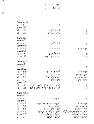
4.6 An Example

Consider the grammar

s --, a [p]

s - , s s

[q]

where q = 1 - p. This highly ambiguous grammar generates strings of any number of a's, using all possible binary parse trees over the given number of terminals. The states

involved in parsing the string

aaa

are listed in Table 2, along with their forward and

inner probabilities. The example illustrates how the parser deals with left-recursion and the merging of alternative sub-parses during completion.

Since the grammar has only a single nonterminal, the left-corner matrix

PL

has

rank 1:

PL = M-

Its transitive closure is

RL = ( I -

PL) -1 ~- ~]-1 ~--- ~/9-1].

Consequently, the example trace shows the factor p-1 being introduced into the for- ward probability terms in the prediction steps.

The sample string can be parsed as either

(a(aa))

or

((aa)a),

each parse having a

probability of

p3q2.

The total string probability is thus 2p3q 2, the computed c~ and 7

values for the final state. The oe values for the scanned states in sets 1, 2, and 3 are

the prefix probabilities for

a, aa,

and

aaa,

respectively: P(S GL a) = 1, P(S

:GL aa) = q,

C o m p u t a t i o n a l Linguistics Volume 21, N u m b e r 2

T a b l e 2

Earley chart as c o n s t r u c t e d d u r i n g the parse of aaa w i t h the g r a m m a r in (a). The t w o c o l u m n s to the right i n (b) list the f o r w a r d a n d i n n e r probabilities, respectively, for each state. In b o t h c~ a n d 3' c o l u m n s , the • separates old factors from n e w o n e s (as p e r e q u a t i o n s 11, 12 a n d 13). A d d i t i o n indicates m u l t i p l e d e r i v a t i o n s of the s a m e state.

(a)

(b)

S ----~ a [p]

S ~ S S [q]

State set 0

0 ~ . S 1 1

predicted

oS ~ .a 1 . p - l p = 1 p

oS ~ .SS 1 • p - l q = p - l q q

State set 1 scanned

oS --* a. p - l p = 1 p

completed

oS --* S . S p - l q . p = q q . p = pq predicted

1S ---* .a q . p - l p = q p

1S ~ .SS q . p - l q = p - l q 2 q

State set 2 scanned

1S ---~ a. q p

completed

1S ~ S . S p - l q 2 , p = q2 q . q = pq

oS ~ SS. q . p = pq pq . p = p2q

oS --* S . S p - l q . p2q = pq2 q . p2q = p2q2 0 ~ S. 1 • p2q = p2q 1 • p2q = p2q predicted

2S ~ .a (q2 q_ pq2) . p - l p = (1 + p)q2 p 2S ~ .SS (q2 q_ pq2) . p - l q = (1 + p-1)q3 q

State set 3 scanned

2S ---* a. (1 -t- p)q2 p

completed

2S ----+ S.S (1 + p-1)q3, p = (1 + p)q3 q . p = pq

[image:18.468.42.415.148.640.2]

4.7 Null Productions

Null productions X --* c introduce some complications into the relatively straight- forward parser operation described so far, some of which are due specifically to the probabilistic aspects of parsing. This section summarizes the necessary modifications to process null productions correctly, using the previous description as a baseline. Our treatment of null productions follows the (nonprobabilistic) formulation of Graham, Harrison, and Ruzzo (1980), rather than the original one in Earley (1970).

4.7.1 Computing c-expansion probabilities. The main problem with null productions is that they allow multiple prediction-completion cycles in between scanning steps (since null productions do not have to be matched against one or more input symbols). Our strategy will be to collapse all predictions and completions due to chains of null productions into the regular prediction and completion steps, not unlike the w a y recursive predictions/completions were handled in Section 4.5.

A prerequisite for this approach is to precompute, for all nonterminals X, the prob- ability that X expands to the empty string. Note that this is another recursive problem, since X itself may not have a null production, but expand to some nonterminal Y that does.

Computation of P ( X :~ c) for all X can be cast as a system of non-linear equations, as follows. For each X, let ex be an abbreviation for P ( X G c). For example, let X have productions

X ---* c [Pl] --* YI Y2 ~92]

---9 W 3 Y 4 Y 5

~/93]

The semantics of context-free rules imply that X can only expand to c if all the RHS nonterminals in one of X's productions expand to e. Translating to probabilities, we obtain the equation

ex -- Pl + p2eyley2 + p3ey3eY4eY5 + "" •

In other words, each production contributes a term in which the rule probability is multiplied by the product of the e variables corresponding to the RHS nonterminals, unless the RHS contains a terminal (in which case the production contributes nothing to ex because it cannot possibly lead to e).

The resulting nonlinear system can be solved by iterative approximation. Each variable ex is initialized to P ( X ~ e), and then repeatedly updated by substituting in the equation right-hand sides, until the desired level of accuracy is attained. Conver- gence is guaranteed, since the ex values are monotonically increasing and bounded above by the true values P ( X ~ e) ( 1. For grammars without cyclic dependen- cies among e-producing nonterminals, this procedure degenerates to simple backward substitution. Obviously the system has to be solved only once for each grammar.

The probability ex can be seen as the precomputed inner probability of an expan- sion of X to the empty string; i.e., it sums the probabilities of all Earley paths that derive c from X. This is the justification for the w a y these probabilities can be used in modified prediction and completion steps, described next.

Computational Linguistics Volume 21, Number 2

are reachable from X by way of the X --*L Y relation. This reachability criterion has to be extended in the presence of null productions. Specifically, if X has a production

X --+ Y1 ...Wi-lYi)~ then Yi is a left corner of X iff Y 1 , . . . , Y i - 1 all have a nonzero probability of expanding to e. The contribution of such a production to the left-corner

probability P ( X --+L Yi) is

i--1

P ( X --* Y 1 . . . Yi-lYi&) I I eYk

k = l

The old prediction procedure can now be modified in two steps. First, replace

the old PL relation by the one that takes into account null productions, as sketched

above. From the resulting PL compute the reflexive transitive closure RL, and use it to

generate predictions as before.

Second, when predicting a left corner Y with a production Y --* Y1 . . . Yi-IYi)~, add

states for all dot positions up to the first RHS nonterminal that cannot expand to e, say from X --* .Y1 . . . Y i - I Yi )~ through X --* Y1 . . . Y i - l . Y i .X. We will call this procedure "spontaneous dot shifting." It accounts precisely for those derivations that expand the

RHS prefix Y1 ... Wi-1 without consuming any of the input symbols.

The forward and inner probabilities of the states thus created are those of the

first state X --* . Y 1 . . . Yi-lYi/~, multiplied by factors that account for the implied e-

expansions. This factor is just the product 1-I~=1 eYk, where j is the dot position.

4.7.3

Completion with null productions.

Modification of the completion step follows

a similar pattern. First, the unit production relation has to be extended to allow for

unit production chains due to null productions. A rule X ~ Y1 . . . Y i - l Y i Y i + l . . . Yj can

effectively act as a unit production that links X and Yi if all other nonterminals on the

RHS can expand to e. Its contribution to the unit production relation P ( X ~ Yi) will

then be

P ( X ~ Y 1 . . . Y i - l Y i Y i + l . . . Yj) I I e Y k

From the resulting revised Pu matrix we compute the closure Ru as usual.

The second modification is another instance of spontaneous dot shifting. When completing a state X --+ )~.Y# and moving the dot to get X ~ )~Y.#, additional states have to be added, obtained by moving the dot further over any nonterminals in # that have nonzero e-expansion probability. As in prediction, forward and inner probabilities are multiplied by the corresponding e-expansion probabilities.

4.7.4 Eliminating null productions. Given these added complications one might con- sider simply eliminating all c-productions in a preprocessing step. This is mostly straightforward and analogous to the corresponding procedure for nonprobabilistic CFGs (Aho and Ullman 1972, Algorithm 2.10). The main difference is the updating of rule probabilities, for which the e-expansion probabilities are again needed.

.

.

Delete all null productions, except on the start symbol (in case the grammar as a whole produces c with nonzero probability). Scale the remaining production probabilities to sum to unity.

(a)

(b)

(c)

Create a variant rule X --* &#

Set the rule probability of the new rule to

eyP(X --, &Y#).

If the rule X ~ ~# already exists, sum the probabilities.

Decrement the old rule probability by the same amount.

Iterate these steps for all RHS occurrences of a null-able nonterminal.

The crucial step in this procedure is the addition of variants of the original produc- tions that simulate the null productions by deleting the corresponding nonterminals from the RHS. The spontaneous dot shifting described in the previous sections effec- tively performs the same operation on the fly as the rules are used in prediction and completion.

4.8 Complexity Issues

The probabilistic extension of Earley's parser preserves the original control structure in most aspects, the major exception being the collapsing of cyclic predictions and unit completions, which can only make these steps more efficient. Therefore the complexity analysis from Earley (1970) applies, and we only summarize the most important results here.

The worst-case complexity for Earley's parser is dominated by the completion step, which takes O(/2) for each input position, I being the length of the current prefix. The total time is therefore O(/3) for an input of length l, which is also the complexity of the standard Inside/Outside (Baker 1979) and LRI (Jelinek and Lafferty 1991) algorithms. For grammars of bounded ambiguity, the incremental per-word cost reduces to O(l), 0(/2) total. For deterministic CFGs the incremental cost is constant, 0(l) total. Because of the possible start indices each state set can contain

0(l)

Earley states, giving O(/2) worst-case space complexity overall.

Apart from input length, complexity is also determined by grammar size. We will not try to give a precise characterization in the case of sparse grammars (Ap- pendix B.3 gives some hints on how to implement the algorithm efficiently for such grammars). However, for fully parameterized grammars in CNF we can verify the scaling of the algorithm in terms of the number of nonterminals n, and verify that it has the same O(n 3) time and space requirements as the Inside/Outside (I/O) and LRI algorithms.

The completion step again dominates the computation, which has to compute probabilities for at most O(n 3) states. By organizing summations (11) and (12) so that 3'" are first summed by LHS nonterminals, the entire completion operation can be accomplished in 0(//3). The one-time cost for the matrix inversions to compute the left-corner and unit production relation matrices is also O(r/3).

5. Extensions

Computational Linguistics Volume 21, Number 2

5.1 Viterbi Parses

Definition 7

A Viterbi parse for a string x, in a grammar G, is a left-most derivation that assigns maximal probability to x, among all possible derivations for x.

Both the definition of Viterbi parse and its computation are straightforward gener- alizations of the corresponding notion for Hidden Markov Models (Rabiner and Juang

1986), where one computes the Viterbi path (state sequence) through an HMM. Pre-

cisely the same approach can be used in the Earley parser, using the fact that each derivation corresponds to a path.

The standard computational technique for Viterbi parses is applicable here. Wher- ever the original parsing procedure sums probabilities that correspond to alternative derivations of a grammatical entity, the summation is replaced by a maximization. Thus, during the forward pass each state must keep track of the maximal path prob- ability leading to it, as well as the predecessor states associated with that maximum probability path. Once the final state is reached, the maximum probability parse can be recovered by tracing back the path of "best" predecessor states.

The following modifications to the probabilistic Earley parser implement the for- ward phase of the Viterbi computation.

• Each state computes an additional probability, its Viterbi probability v.

• Viterbi probabilities are propagated in the same way as inner

probabilities, except that during completion the summation is replaced

by maximization: Vi(kX --* ,~Y.#) is the maximum of all products

vi(jW --+ 17.)Vj(kX --+ ,~.Y#) that contribute to the completed state

kX --* )~Y.#. The same-position predecessor j Y -~ ~,. associated with the

maximum is recorded as the Viterbi path predecessor of kX --* ,~Y.# (the

other predecessor state kX --* ,~.Y# can be inferred).

• The completion step uses the original recursion without collapsing unit

production loops. Loops are simply avoided, since they can only lower a path's probability. Collapsing unit production completions has to be avoided to maintain a continuous chain of predecessors for later backtracing and parse construction.

• The prediction step does not need to be modified for the Viterbi

computation.

Once the final state is reached, a recursive procedure can recover the parse tree associated with the Viterbi parse. This procedure takes an Earley state i : kX --* &.# as input and produces the Viterbi parse for the substring between k and i as output. (If the input state is not complete (# ~ ¢), the result will be a partial parse tree with children missing from the root node.)

Viterbi parse (i : k X --* -~.#):

. Otherwise, if ~ ends in a terminal a, let A~a = ~, and call this procedure recursively to obtain the parse tree

T = Viterbi-parse(i - 1 : k X i+ ,,V.a~)

.

Adjoin a leaf node labeled a as the right-most child to the root of T and return T.

Otherwise, if A ends in a nonterminal Y, let A'Y = A. Find the Viterbi

predecessor state jW ---+ t~. for the current state. Call this procedure

recursively to compute

T = Viterbi-parse(j : kX ~ A'.Y#)

as well as

T' = Viterbi-parse(i : jY --* u.)

Adjoin T ~ to T as the right-most child at the root, and return T.

5.2 Rule Probability Estimation

The rule probabilities in a SCFG can be iteratively estimated using the EM (Expectation- Maximization) algorithm (Dempster et al. 1977). Given a sample corpus D, the esti- mation procedure finds a set of parameters that represent a local maximum of the

grammar likelihood function P(D I G), which is given by the product of the string

probabilities

P(D I C) = 1-[ P(S

x),

xED

i.e., the samples are assumed to be distributed identically and independently. The two steps of this algorithm can be briefly characterized as follows.

E-step: Compute expectations for how often each grammar rule is used, given the corpus D and the current grammar parameters (rule probabilities).

M-step:

Reset the parameters so as to maximize the likelihood relative to the expected rule counts found in the E-step.

This procedure is iterated until the parameter values (as well as the likelihood) con- verge. It can be shown that each round in the algorithm produces a likelihood that is at least as high as the previous one; the EM algorithm is therefore guaranteed to find at least a local maximum of the likelihood function.

EM is a generalization of the well-known Baum-Welch algorithm for HMM esti- mation (Baum et al. 1970); the original formulation for the case of SCFGs is attributable to Baker (1979). For SCFGs, the E-step involves computing the expected number of times each production is applied in generating the training corpus. After that, the M- step consists of a simple normalization of these counts to yield the new production probabilities.

Computational Linguistics Volume 21, Number 2

Definition 8

Given a string x, Ix] = l, the outer probability fli(kX ---* A.#) of an Earley state is the

s u m of the probabilities of all paths that

.

2.

3.

4.

5.

start with the initial state,

generate the prefix X o . . . X k - 1 ,

pass t h r o u g h k x ---4 .17#, for some u,

generate the suffix xi. • • x1-1 starting with state kX --* u.# ,

end in the final state.

Outer probabilities complement inner probabilities in that they refer precisely to those parts of complete paths generating x not covered by the corresponding inner

probability 7i(kX --* A.#). Therefore, the choice of the production X --* A# is not part

of the outer probability associated with a state kX ~ A.#. In fact, the definition makes

no reference to the first part A of the RHS: all states sharing the same k, X, a n d # will have identical outer probabilities.

Intuitively, fli(kX --* A.#) is the probability that an Earley parser operating as a

string generator yields the prefix Xo...k-1 a n d the suffix xi...l_l, while passing t h r o u g h

state kX --* A.# at position i (which is i n d e p e n d e n t of A). As was the case for forward

probabilities, fl is actually an expectation of the n u m b e r of such states in the path, as unit production cycles can result in multiple occurrences for a single state. Again, we gloss over this technicality in our terminology. The n a m e is motivated b y the fact that fl reduces to the "outer probability" of X, as defined in Baker (1979), if the dot is in final position.

5.2.1 C o m p u t i n g expected production counts. Before going into the details of com-

p u t i n g outer probabilities, we describe their use in obtaining the expected rule counts needed for the E-step in g r a m m a r estimation.

Let c ( X --* A ] x) denote the expected n u m b e r of uses of production X --* A in the

derivation of string x. Alternatively, c ( X --* A ] x) is the expected n u m b e r of times that

X --+ ), is used for prediction in a complete Earley path generating x. Let c ( X -~ A ] t 9)

be the n u m b e r of occurrences of predicted states based on production X ~ A along a path 79.

c(x

lx)

=

Z

P(791s x)c(X

;,

179)

79 derives x

1

-

F_,

p(79, s

x)c(x

P(S ~ x) 79 derives x

_ 1

P(S ~ Xo...i_lXl] ~ x). P(S _{X) i:iX---+.A}

79)

The last s u m m a t i o n is over all predicted states based on production X --* A. The

quantity P(S • Xo...i_lXt, :~ x) is the s u m of the probabilities of all paths passing

through i : iX --* .A. Inner a n d outer probabilities have been defined such that this