Grounding Language with Points and Paths in Continuous Spaces

Grounding Language with Points and Paths in Continuous Spaces

Jacob Andreas and Dan Klein

Computer Science Division University of California, Berkeley

{jda,klein}@cs.berkeley.edu

Abstract

We present a model for generating path-valued interpretations of natural language text. Our model encodes a map from natural language descriptions to paths, mediated by segmentation variables which break the language into a discrete set of events, and alignment variables which reorder those events. Within an event, lexical weights capture the contribution of each word to the aligned path segment. We demonstrate the applicability of our model on three diverse tasks: a new color description task, a new financial news task and an established direction-following task. On all three, the model outperforms strong baselines, and on a hard variant of the direction-following task it achieves results close to the state-of-the-art system described in Vogel and Jurafsky (2010).

1 Introduction

This paper introduces a probabilistic model for predicting grounded, real-valued trajectories from natural language text. A long tradition of re-search in compositional semantics has focused on discrete representations of meaning. The origi-nal focus of such work was on logical translation: mapping statements of natural language to a for-mal language like first-order logic (Zettlemoyer and Collins, 2005) or database queries (Zelle and Mooney, 1996). Subsequent work has integrated this logical translation with interpretation against a symbolic database (Liang et al., 2013).

There has been a recent increase in interest in perceptual grounding, where lexical semantics anchor in perceptual variables (points, distances, etc.) derived from images or video. Bruni et al. (2014) describe a procedure for constructing word representations using text- and image-based

dis-% Cha

nge

0.98 0.99 1.00 1.01 1.02

Hour of day

10 12 14 10 12 14

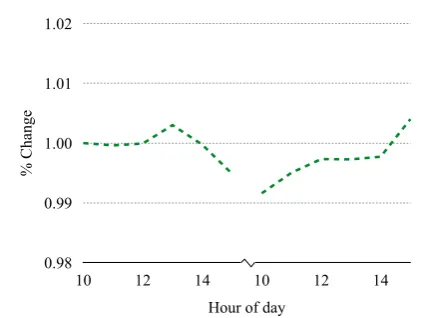
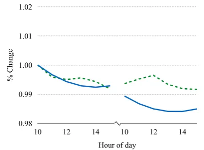
U.S. stocks rebound after bruising two-day swoon Figure 1: Example stock data. The chart displays index value over a two-day period (divided by the dotted line), while the accompanying headline de-scribes the observed behavior.

tributional information. Yu and Siskind (2013) describe a model for identifying scenes given de-scriptions, and Golland et al. (2010), Kollar et al. (2010), and Krishnamurthy and Kollar (2013) de-scribe models for identifying individual compo-nents of scenes described by text. These all have the form of matching problems between text and observed groundings—what has been missing so far is the ability togenerategrounded interpreta-tions from scratch, given only text.

Our work continues in the tradition of this per-ceptual grounding work, but makes two contribu-tions. First, our approach is able to predict simple world states (and their evolution): for a general class of continuous domains, we produce a repre-sentation ofp(world|text)that admits easy sam-pling and maximization. This makes it possible to produce grounded interpretations of text without reference to a pre-existing scene. Simultaneously, we extend the range of temporal phenomena that can be modeled—unlike the aforementioned spa-tial semantics work, we consider language that

scribes time-evolving trajectories, and unlike Yu and Siskind (2013), we allow these trajectories to have event substructure, and model temporal or-dering. Our class of models generalizes to a vari-ety of different domains: a new color-picking task, a new financial news task, and a more challenging variant of the direction-following task established by Vogel and Jurafsky (2010).

As an example of the kinds of phenomena we want to model, consider Figure 1, which shows the value of the Dow Jones Industrial Average over June 3rd and 4th 2008, along with a finan-cial news headline from June 4th. There are sev-eral effects of interest here. One phenomenon we want to capture is that the lexical semantics of in-dividual words must be combined:swoonroughly describes a drop whilebruisingindicates that the drop was severe. We isolate this lexical combi-nation in Section 4, where we consider a limited model of color descriptions (Figure 2). A second phenomenon is that the description is composed of two separate events, a swoon and a rebound; moreover, those events do not occur in their tex-tual order, as revealed byafter. In Section 5, we extend the model to include segmentation and or-dering variables and apply it to this stock data.

The situation where language describes a path through some continuous space—literal or metaphorical—is more general than stock head-lines. Our claim is that a variety of problems in language share these same characteristics. To demonstrate generality of the model, we also ap-ply it in Section 6 to a challenging variant of the direction-following task described by Vogel and Jurafsky (2010) (Figure 3), where we achieve re-sults close to a state-of-the-art system that makes stronger assumptions about the task.

2 Three tasks in grounded semantics

The problem of inferring a structured state repre-sentation from sensory input is a hard one, but we can begin to tackle grounded semantics by restrict-ing ourselves to cases where we have sequences of real-valued observations directly described by text. In this paper we’ll consider the problems of recognizing colors, describing time series, and following navigational instructions. While these tasks have been independently studied, we believe that this is the first work which presents them in a unified framework, and carries them out with a single family of models.

.

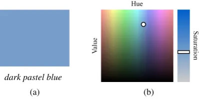
dark pastel blue

(a) (b)

Figure 2: Example color data: (a) a named color; (b) its coordinates in color space.

Colors Figure 2 shows a color calleddark pas-tel blue. English speakers, even if unfamiliar with the specific color, can identify roughly what the name signifies because of prior knowledge of the meanings of the individual words.

Because the color domain exhibits lexical com-positionality but not event structure, we present it here to isolate the non-temporal compositional ef-fects in our model. Any color visible to the human eye can be identified with three coordinates, which we’ll take to be hue, saturation and value (HSV). As can be seen in Figure 2 the “hue” axis corre-sponds to the differentiation made by basic color names in most languages. Other modifiers act on the saturation and value axes: either simple ones likedark(which decreases value), or more compli-cated ones likepastel(which increases value and decreases saturation). Given a set of named colors and their HSV coordinates, a learning algorithm should be able to identify the effects of each word in the vocabulary and predict the appearance of new colors with previously-unseen combinations of modifiers.

Compositional interpretations of color have re-ceived attention in linguistics and philosophy of language (Kennedy and McNally, 2010), but while work in grounded computational semantics like that of Krishnamurthy and Kollar (2013) has suc-ceeded in learning simple color predicates, our model is the first to capture the machine learning of color in a fine-grained, compositional way.

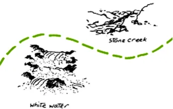
Head-right round the white water [. . . ] but stay quite close ’cause you don’t otherwise you’re going to be in that stone creek Figure 3: Example map data: a portion of a map, and a single line from a dialog which describes navigation relative to the two visible landmarks.

lines may describe multiple events, or multi-part events likereboundorextend; stocks do not sim-plyriseorfall, but stagger,stumble, swoon, and so on. There are compositional effects here as well: distinction is made between falling and

falling sharply; gradual trends are distinguished from those which occur suddenly, at the beginning or end of the trading day. Along with temporal structure, the problem requires a more sophisti-cated treatment of syntax than the colors case— now we have to identify which subspans of the sentence are associated with each event observed, and determine the correspondence between sur-face order and actual order in time.

The learning of correspondences between text and time series has attracted more interest in nat-ural language generation than in semantics (Yu et al., 2007). Research on natural language process-ing and stock data, meanwhile, has largely focused on prediction of future events (Kogan et al., 2009).

Direction following We’ll conclude by

apply-ing our model to the well-studied problem of following navigational directions. A variety of reinforcement-learning approaches for following directions on a map were previously investigated by Vogel and Jurafsky (2010) using a corpus as-sembled by Anderson et al. (1991). An example portion of a path and its accompanying instruction is shown in Figure 3. While also representable as a set of real valued coordinates, here 2-d, this data set looks very different—a typical example con-sists of more than a hundred sentences of the kind shown in Figure 3, accompanying a long path. The language, a transcript of a spoken dialog, is also

considerably less formal than the language found in theWall Street Journalexamples, involving dis-fluency, redundancy and occasionally errors. Nev-ertheless the underlying structure of this problem and the stock problem are fundamentally similar.

In addition to Vogel and Jurafsky, Tellex et al. (2011) give a weakly-supervised model for map-ping single sentences to commands, and Brana-van et al. (2009) give an alternative reinforcement-learning approach for following long command se-quences. An intermediate between this approach and ours is the work of Chen and Mooney (2011) and Artzi and Zettlemoyer (2013), which boot-strap a semantic parser to generate logical forms specifying the output path, rather than predicting the path directly.

Between them, these tasks span a wide range of linguistic phenomena relevant to grounded seman-tics, and provide a demonstration of the useful-ness and general applicability of our model. While development of the perceptual groundwork neces-sary to generalize these results to more complex state spaces remains a major problem, our three examples provide a starting point for studying the relationship between perception, time and the se-mantics of natural language.

3 Preliminaries

In the experiments that follow, each training ex-ample will consist of:

– Natural language text, consisting of a con-stituency parse tree or trees. For a given ex-ample, we will denote the associated trees (T1,T2, . . .). These are also observed at test

time, and used to predict new groundings. – A vector-valued, grounded observation, or

a sequence of observations (a path), which we will denote V for a given example. We will further assume that each of these paths has been pre-segmented (discussed in detail in Section 5) into a sequence (V1,V2, . . .).

These are only observed during training. The probabilistic backbone of our model is a collection of linear and log-linear predictors. Thus it will be useful to work with vector-valued rep-resentations of both the language and the path, which we accomplish with a pair of feature func-tions ϕt and ϕv. As the model is defined only

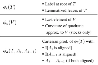
ϕt(T)

■Label at root ofT ■Lemmatized leaves ofT

ϕv(V)

■Last element ofV ■Curvature of quadratic

approx. toV (stocks only)

ϕa(T, Ai, Ai−1)

Cartesian prod. ofϕt(T)with:

■I[A

iis aligned]

■I[A_i−1is aligned]

■A₁−A_i−1(if both aligned)

Table 1: Features used for linear parameterization of the grounding model.

simplify notation by writing Ti = ϕt(Ti) and Vi =ϕv(Vi). As the ultimate prediction task is to

produce paths, and not their featurized representa-tions, we will assume that it is also straightforward to computeϕ−1

v , which projects path features back

into the original grounding domain.

All parse trees are predicted from input text us-ing the Berkeley Parser (Petrov and Klein, 2007). Feature representations for both trees and paths are simple and largely domain-independent; they are explicitly enumerated in Table 1.

The general framework presented here leaves one significant problem unaddressed: given a large state vector encoding properties of multiple ob-jects, how do we resolve an utterance about a sin-gle object to the correct subset of indices in the vector? While none of the tasks considered in this paper require an argument resolution step of this kind, interpretation of noun phrases is one of the better-studied problems in compositional seman-tics (Zelle and Mooney (1996), inter alia), and we expect generalization of this approach to be straightforward using these tools.

We will consider the color, stock, and naviga-tion tasks in turn. It is possible to view the models we give for all three as instantiations of the same graphical model, but for ease of presentation we will introduce this model incrementally.

4 Predicting vectors

Prediction of a color variable from text has the form of a regression problem: given a vector of lexical features extracted from the name, we wish to predict the entries of a vector in color space. It seems linguistically plausible that this regression issparseandlinear: that most words, if they pro-vide any constraints at all, tend to express

prefer-ences about a subset of the available dimensions; and that composition within the domain of a sin-gle event largely consists of words additively pre-dicting that event’s parameters, without complex nonlinear interactions. This is motivated by the observation that pragmatic concerns force linguis-tic descriptors to orient themselves along a small set of perceptual bases: once we have words for

northandeast, we tend to describe intermediates as northeast rather than inventing an additional word which means “a little of both”.

As discussed above, we can represent a color as a point in a three-dimensional HSV space. LetT

denote features on the parse tree of the color name, andV its representation in color space (consistent with the definition ofϕvgiven in Table 1).

Linear-ity suggests the following model:

p(T, V)∝e−∥θt⊤T−V∥2₂ (1)

The learning problem is then:

argmin

θt

∑

T,V

θ⊤_t T−V2

2 (2)

which, with a sparse prior on θt, is the

proba-bilistic formulation of Lasso regression (Tibshi-rani, 1996), for which standard tools are available in the optimization literature.

To predict color space values from a new (fea-turized) nameT, we output:

argmax

V p(T, V) =θ

⊤

t T

4.1 Evaluation

We collect a set of color names and their corresponding HSV triples from the English Wikipedia’s List of Colors, retaining only those color names in which every word appears at least three times in the training corpus. This leaves a set of 419 colors, which we randomly divide into a 377-item training set and 42-item test set. The model’s goal will be to learn to identify new col-ors given only their names.

Method Sel.↑ H↓ S↓ V↓

Random 0.50 0.30 0.38 0.39 Last word 0.78 0.05 0.26 0.17 Full model 0.81 0.07 0.21 0.13

Human 0.86 - -

-Table 2: Results for the color selection task. Sel(ection accuracy) is frequency with which the system was able to correctly identify the color de-scribed when paired with a random alternative. Other columns are the magnitude of the average prediction error along the axes of the color space. Full model selection accuracy is a statistically sig-nificant (p <0.05) improvement over the baseline using a paired sign test.

the color corresponding to the name and another drawn randomly from the test set, and report the fraction of times the true color is assigned a higher probability than the random alternative. In the sec-ond, we report the absolute value of the difference between true and predicted hue, saturation, and lu-minosity.

We compare against two baselines: one which looks only at the last word in the color name (al-most always a hue category), and so captures no compositional effects, and another which outputs random values for all three coordinates. Results are shown in Table 2. The model with all lexical features outperforms both baselines on selection and all but one absolute error metric.

4.2 Error analysis

An informal experiment in which the color selec-tion task was repeated on one of the authors’ col-leagues (the “Human” row in Table 2) yielded an accuracy of 86%, only 5% better than the system. While not intended as a rigorous upper bound on performance, this suggests that the model capac-ity and training data are sufficient to capture most interesting color behavior. The errors that do oc-cur appear to mostly be of two kinds. In one case, a base color is seen only with a small (or related) set of modifiers, from which the system is unable to infer the meaning of the base color (e.g. from

Japanese indigo,lavender indigo, andelectric in-digo, the learning algorithm infers that indigo is bright purple). In the other, no part of the color word is seen in training, and the system outputs an unrelated “default” color (teal is predicted to be bright red).

5 Predicting paths

The idea that a sentence’s meaning is fundamen-tally described by a set ofevents, each associated with a set of predicates, is well-developed in neo-Davidsonian formal semantics (Parsons, 1990). We adopt the skeleton of this formal approach by tying our model to (latent) partitions of the in-put sentence into disjoint events. Rather than at-tempting to pass through a symbolic meaning rep-resentation, however, this event structure will be used to map text directly into the grounding do-main. We assume that this domain has pre-existing structure—in particular, that in our input pathsV, the boundaries of events have already been iden-tified, and that the problem of aligning text to portions of the segment only requires aligning to segment indices rather than fine-grained time in-dices. This is a strong assumption, and one that future work may wish to revisit, but there exist both computational tools from the changepoint de-tection literature (Basseville and Nikiforov, 1995) and pieces of evidence from cognitive science (Za-cks and Swallow, 2007) which suggest that assum-ing a pre-lassum-inguistic structurassum-ing of events is a rea-sonable starting point.

In the text domain, we make the corresponding assumption that each of these events is syntacti-cally local—that a given span of the input sentence provides information about at most one of these segmented events.

The main structural difference between the color example in Figure 2 and the stock market ex-ample in Figure 1 is the introduction of a time di-mension orthogonal to the didi-mensions of the state space. To accommodate this change, we extend the model described in the previous subsection in the following way: Instead of a single vector, each tree representationT is paired with asequenceof path featuresV= (V1, V2, . . . , VM). For the time

being we continue to assume that there is only one input tree per training example. As before, we wish to model the probabilityp(T,V), but the problem becomes harder: a single sentence might describe multiple events, but we don’t know what the correspondence is between regions of the sen-tence and segmentsV.

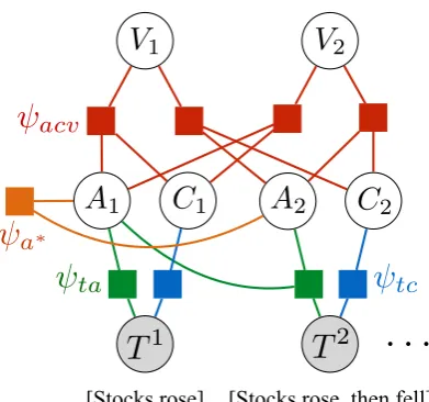
Though the ultimate goal is still prediction ofV

mul-· mul-· mul-·

A

C

A

C2

V

V

T

T

[Stocks rose] [Stocks rose, then fell] acv

a⇤

ta tc

Figure 4: Factor graph for stocks grounding model. Only a subset of the alignment candidates are shown.ψtcmaps text to constraints,ψacvmaps

constraints to grounded segments, andψta

deter-mines which constraints act on which segments.

tiple events, we’ll break eachT apart into a set of

alignment candidatesTi_{. We’ll allow as an}

align-ment candidate any subtree ofT, and additionally any subtree from which a single constituent has been deleted.

We then introduce two groups of latent vari-ables: alignment variables A = (A1, A2, . . .),

which together describe a mapping from pieces of the input sentence to segments of the ob-served path, and what we’ll call “constraint” vari-ables C = (C1, C2, . . .), which express each

aligned tree segment’s prediction about what its corresponding path should look like (so that the possibly-numerous parts of the tree aligned to a single segment can independently express prefer-ences about the segment’s path features).

In addition to ensuring that the alignment is consistent with the bracketing of the tree, it might be desirable to impose additional global con-straints on the alignment. There are various ways to do this in a graphical modeling framework; the most straightforward is to add a combinatorial fac-tor touching all alignment variables which checks for satisfaction of the global constraint. In gen-eral this makes alignment intractable. If the total number of alignments licensed by this combina-torial factor is small (i.e. if acceptable alignments are sparse within the exponentially-large set of all possible assignments to A), it is possible to di-rectly sum them out during inference. Otherwise

approximate techniques (as discussed in the fol-lowing section) will be necessary.

As discussed in Section 2, our financial time-lines cover two-day periods, and it seems natural to treat each day as a separate event. Then the simple regression model described in the preceding section, extended to include alignment and constraint variables, has the form of the factor graph shown in Figure 4. In particular, the joint distributionp(T,V)is the product of four groups of factors:

Alignment factors ψta, which use a log-linear

model to score neighboring pairs of factors with a feature functionϕa:

ψta(Ti, Ai, Ai−1) =

eθ⊤

aϕa(Ti,Ai,Ai−1)

∑

A′

i,A′i−1e

θ⊤_aϕa(Ti_,A′

i,A′i−1) (3)

Constraint factors ψtc, which map text features

onto constraint values:

ψtc(Ti, Ci) =e−||θt⊤Ti−Ci||22 (4)

Prediction factors ψacv which encourage

pre-dicted constraints and path features to agree:

ψacv(Ai, Ci, Vj) =

{

1 ifAi̸=j

e−||Ci−Vj||22 o.w. (5)

A global factor ψa∗(A₁, A₂,· · ·) which places

an arbitrary combinatorial constraint on the alignment.

Note the essential similarity between Equations 1 and 4—in general, it can be shown that this factor model reduces to the regression model we gave for colors when there is only one of eachTi_andVj. 5.1 Learning

In order to make learning in the stocks domain tractable, we introduce the following global constraints on alignment: every terminal must be aligned, and two constituents cannot be aligned to the same segment. Together, these simplify learning by ensuring that the number of terms in the sum over A and Cis polynomial (in fact

O(n2_{)) in the length of the input sentence. We}

wish to find the maximum a posteriori estimate

using the Expectation–Maximization algorithm. To find regression scoring weightsθt, we have:

E step:

M =E

[ ∑

i

Ti_(Ti₎⊤ ]

; N =E

[ ∑

i

Ti_V⊤

Ai

] (6)

M step:

θt=M−1N (7)

To find alignment scoring weights θa, we must

maximize:

∑

i E

 _log



_∑ eθa⊤ϕa(Ai,Ai−1,Ti)

A′

i,A′i−1e

θ⊤_aϕa(A′

i,A′i−1,Ti)

    ₍₈₎

which can be done using a variety of convex op-timization tools; we used L-BFGS (Liu and No-cedal, 1989).

The predictive distributionp(V|T)can also be straightforwardly computed using the standard in-ference procedures for graphical models.

5.2 Evaluation

Our stocks dataset consists of a set of headlines from the “Market Snapshot” column of the Wall Street Journal’s MarketWatch website,1 _paired

with hourly stock charts for each day described in a headline. Data is collected over a roughly decade-long period between 2001 and 2012; af-ter removing weekends and days with incomplete stock data, we have a total of 2218 headline/time series pairs. As headlines most often discuss a single day or a short multi-day period, each train-ing example consists of two days’ worth of stock data concatenated together. We use a 90%/10% train/test split, with all test examples following all training examples chronologically.

We compare against two baselines: one which uses no text (and so learns only the overall mar-ket trend during the training period), and another which uses a fixed alignment instead of summing, aligning the entire tree to the second day’s time se-ries. Prediction error is the sum of squared errors between the predicted and gold time series.

We report both the magnitude of the prediction error, and the model’s ability to distinguish be-tween the described path and a randomly-selected alternative. The system scores poorly on squared

1_{http://www.marketwatch.com/Search?m=}

Column&mp=Market%20Snapshot

% Cha

nge

0.98 0.99 1.00 1.01 1.02

Hour of day

10 12 14 10 12 14

[U.S. stocks end lower]2[as economic worries persist]1

Figure 5: Example output from the stocks task. The model prediction is given in blue (solid), and the reference time series in green (dashed). Brack-ets indicate the predicted boundaries of event-introducing spans, and subscripts their order in the sentence. The model correctly identifies thatend lower refers to the current day, and persist pro-vides information about the previous day.

Method Sel. acc.↑ Pred. err.↓

No text 0.51 0.0012 Fixed alignment 0.59 0.0011

Full model 0.61 0.0018

Human 0.72 –

Table 3: Results for the stocks task. Sel(ection accuracy) measures the frequency with which the system correctly identifies the stock described in the headline when paired with a random alterna-tive. Pred(iction error) is the mean sum of squared errors between the real and predicted paths. Full model selection accuracy is a statistically signif-icant improvement (p < 0.05) over the baseline using a paired sign test.

error (which disproportionately penalizes large de-viations from the correct answer, preferring con-servative models), but outperforms both base-lines on the task of choosing the described stock history—when it is wrong, its errors are often large in magnitude, but its predictions more fre-quently resemble the correct time series than the other systems.

% Cha

nge

0.98 0.99 1.00 1.01 1.02

Hour of day

10 12 14 10 12 14

[U.S. stocks extend losing stretch]1

Figure 6: Example error from the stocks task. The system’s prediction, in blue (solid), fails to seg-ment the input into two events, and thus incor-rectly extends thelosingtrend to the entire output time span.

features learned by the model—as desired, it cor-rectly interprets a variety of different expressions used to describe stock behavior.

5.3 Error analysis

As suggested by Table 4, learned weights for the trajectory-grounded featuresθtare largely correct.

Thus, most incorrect outputs from the system in-volve alignment to time. Many multipart events (likerebound) can be reasonably explained using the curvature feature without splitting the text into two segments; as a result, the system tends to be fairly conservative about segmentation and often under-segments. This results in examples like Fig-ure 6, in which the downward trend suggested by

losing is incorrectly extended to the entire out-put curve. Here, another informal experiment us-ing humans as the predictors indicates that pre-dictions are farther from human-level performance

Word Sign Magnitude·103

rise 0.27 −0.78 swoon −0.57 0 sharply −0.22 0.28 slammed −0.36 0

lifted 0.66 0

Table 4: Learned parameter settings for overall daily change, which the path featurization decom-poses into a sign and a magnitude.

than they are on the colors task.

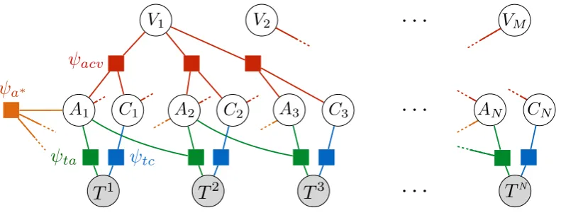
6 Generalizing the model

Last we consider the problem of following navi-gational directions. The difference between this and the previous task is largely one of scale: rather than attempting to predict the values of only two segments, we have a long string of them. The text, rather than a single tree, consists of a sequence of tens or hundreds of pre-segmented utterances.

There is one additional complication—rather than being defined in an absolute space, as they are in the case of stocks, constraints in the maps do-main are provided relative to a set of known land-marks (like thewhite waterandstone creekin Fig-ure 3). We resolve landmarks automatically based on string matching, in a manner similar to Vogel and Jurafsky (2010), and assign each sentence in the discourse with a single referred-to landmarkli.

If no landmark is explicitly named, it inherits from the previous utterance. We continue to score con-straints as before, but update the prediction factor:

ψacv(Ai, Ci, Vj) =

{

1 ifAi ̸=j

e−||li+Ci−Vj||22 o.w. (9)

The factor graph is shown in Figure 7; ob-serve that this is simply an unrolled version of Figure 4—the basic structure of the model is un-changed. While pre-segmentation of the discourse means we can avoid aligning internal constituents of trees, we still need to treat every utterance as an alignment candidate, without a sparse combinato-rial constraint. As a result, the sum over A and Cis no longer tractable to compute explicitly, and approximate inference will be necessary.

For the experiments described in this paper, we do this with a sequence of Monte Carlo approxi-mations. We run a Gibbs sampler, iteratively re-sampling eachAiandCias well as the parameter

vectors θt andθa to obtain estimates of Eθt and Eθa. The resampling steps forθtandθaare

them-selves difficult to perform exactly, so we perform an internal Metropolis-Hastings run (with a Gaus-sian proposal distribution) to obtain samples from the marginal distributions overθtandθa.

· · ·

· · ·

· · ·

C

A

A

C

A

C

A

C

V

V

V

T

T

T

T

ta tc

a⇤

acv

Figure 7: Factor graph for the general grounding model. Note that Figure 4 is a subgraph.

we must invertϕv, which we do by producing the

shortest path licensed by the features.

6.1 Evaluation

The Map Task Corpus consists of 128 dia-logues describing paths on 16 maps, accompa-nied by transcriptions of spoken instructions, pre-segmented using prosodic cues. See Vogel and Ju-rafsky (2010) for a more detailed description of the corpus in a language learning setting. For com-parability, we’ll use the same evaluation as Vogel and Jurafsky, which rewards the system for mov-ing between pairs of landmarks that also appear in the reference path, and penalizes it for additional superfluous movement. Note that we are solv-ing a significantly harder problem: the version ad-dressed by Vogel and Jurafsky is a discrete search problem, and the system has hard-coded knowl-edge that all paths pass along one of the four sides of each landmark. Our system, by contrast, can navigate to any point inR2_{, and must learnthat}

most paths stay close to a named landmark. At test time, the system is given a new sequence of text instructions, and must output the corre-sponding path. It is scored on the fraction of correct transitions in its output path (precision), and the fraction of transitions in the gold path recovered (recall). Vogel and Jurafsky compare their system to a policy-gradient algorithm for us-ing language to follow natural language instruc-tions described by Branavan et al. (2009), and we present both systems for comparison.

Results are shown in Table 5. Our system sub-stantially outperforms the policy gradient baseline of Branavan et al., and performs close (particularly with respect to transition recall) to the system of Vogel and Jurafsky, with fewer assumptions.

System Prec. Recall F1

Branavan et al. (09) 0.31 0.44 0.36 Vogel & Jurafsky (10) 0.46 0.51 0.48 This work 0.43 0.51 0.45

Table 5: Results for the navigation task. Higher is better for all of precision, recall andF1.

6.2 Error analysis

As in the case of stocks, most of the prediction errors on this task are a result of misalignment. In particular, many of the dialogues make passing reference to already-visited landmarks, or define destinations in empty regions of the map in terms of multiple landmarks simultaneously. In each of these cases, the system is prone to directly visit-ing the named landmark or landmarks instead of ignoring or interpolating as necessary.

7 Conclusion

We have presented a probabilistic model for grounding natural language text in vector-valued state sequences. The model is capable of seg-menting text into a series of events, ordering these events in time, and compositionally determining their internal structure. We have evaluated on a va-riety of new and established applications involving colors, time series and navigation, demonstrating improvements over strong baselines in all cases.

Acknowledgments

References

Anne H Anderson, Miles Bader, Ellen Gurman Bard, Elizabeth Boyle, Gwyneth Doherty, Simon Garrod, Stephen Isard, Jacqueline Kowtko, Jan McAllister, Jim Miller, et al. 1991. The HCRC map task corpus. Language and speech, 34(4):351–366.

Yoav Artzi and Luke Zettlemoyer. 2013. Weakly su-pervised learning of semantic parsers for mapping instructions to actions. Transactions of the Associa-tion for ComputaAssocia-tional Linguistics, 1(1):49–62.

Michele Basseville and Igor V Nikiforov. 1995. De-tection of abrupt changes: theory and applications. Journal of the Royal Statistical Society-Series A Statistics in Society, 158(1):185.

SRK Branavan, Harr Chen, Luke S Zettlemoyer, and Regina Barzilay. 2009. Reinforcement learning for mapping instructions to actions. InProceedings of the Joint Conference of the 47th Annual Meeting of the ACL and the 4th International Joint Conference on Natural Language Processing of the AFNLP: Vol-ume 1-VolVol-ume 1, pages 82–90. Association for Com-putational Linguistics.

Elia Bruni, Nam Khanh Tran, and Marco Baroni. 2014. Multimodal distributional semantics. Journal of Ar-tificial Intelligence Research, 49:1–47.

David L Chen and Raymond J Mooney. 2011. Learn-ing to interpret natural language navigation instruc-tions from observainstruc-tions. InAAAI, volume 2.

Dave Golland, Percy Liang, and Dan Klein. 2010. A game-theoretic approach to generating spatial de-scriptions. InProceedings of the 2010 conference on Empirical Methods in Natural Language Process-ing, pages 410–419. Association for Computational Linguistics.

Christopher Kennedy and Louise McNally. 2010. Color, context, and compositionality. Synthese, 174(1):79–98.

Shimon Kogan, Dimitry Levin, Bryan R Routledge, Jacob S Sagi, and Noah A Smith. 2009. Pre-dicting risk from financial reports with regression. In Proceedings of Human Language Technologies: The 2009 Annual Conference of the North American Chapter of the Association for Computational Lin-guistics, pages 272–280. Association for Computa-tional Linguistics.

Thomas Kollar, Stefanie Tellex, Deb Roy, and Nicholas Roy. 2010. Grounding verbs of motion in natu-ral language commands to robots. In International Symposium on Experimental Robotics.

Jayant Krishnamurthy and Thomas Kollar. 2013. Jointly learning to parse and perceive: connecting natural language to the physical world.Transactions of the Association for Computational Linguistics.

Percy Liang, Michael I Jordan, and Dan Klein. 2013. Learning dependency-based compositional seman-tics. Computational Linguistics, 39(2):389–446. Dong C Liu and Jorge Nocedal. 1989. On the limited

memory BFGS method for large scale optimization. Mathematical programming, 45(1-3):503–528. Terence Parsons. 1990. Events in the semantics of

En-glish. MIT Press.

Slav Petrov and Dan Klein. 2007. Improved inference for unlexicalized parsing. InProceedings of Human Language Technologies: The 2007 Annual Confer-ence of the North American Chapter of the Associ-ation for ComputAssoci-ational Linguistics. AssocAssoci-ation for Computational Linguistics.

Stefanie Tellex, Thomas Kollar, Steven Dickerson, Matthew R. Walter, Ashis Gopal Banerjee, Seth Teller, and Nicholas Roy. 2011. Understanding nat-ural language commands for robotic navigation and mobile manipulation. InIn Proceedings of the Na-tional Conference on Artificial Intelligence. Robert Tibshirani. 1996. Regression shrinkage and

se-lection via the lasso. Journal of the Royal Statistical Society. Series B (Methodological), pages 267–288. Adam Vogel and Dan Jurafsky. 2010. Learning to fol-low navigational directions. In Proceedings of the 48th Annual Meeting of the Association for Compu-tational Linguistics, pages 806–814. Association for Computational Linguistics.

Haonan Yu and Jeffrey Mark Siskind. 2013. Grounded language learning from videos described with sen-tences. In Proceedings of the 51st Annual Meet-ing of the Association for Computational LMeet-inguis- Linguis-tics. Association for Computational LinguisLinguis-tics. Jin Yu, Ehud Reiter, Jim Hunter, and Chris Mellish.

2007. Choosing the content of textual summaries of large time-series data sets. Natural Language Engi-neering, 13(1):25–49.

Jeffrey M Zacks and Khena M Swallow. 2007. Event segmentation. Current Directions in Psychological Science, 16(2):80–84.

John M Zelle and Raymond J Mooney. 1996. Learn-ing to parse database queries usLearn-ing inductive logic programming. InProceedings of the National Con-ference on Artificial Intelligence, pages 1050–1055. Luke S. Zettlemoyer and Michael Collins. 2005.