Teaming up drivers
A pilot study on social navigation.
Bachelor Thesis
Alje van den Bosch,
Berkeley, October 30, 2008
Acknowledgements
After 10 weeks of working here at Path I’m happy to present the result of my research. Living and working in a foreign environment has taught me more than I can convey in this document. I saw a lot of the projects going on and met a lot of people. The research was hard from time to time because sometimes it seemed more than I could handle. I couldn’t do everything as perfect as I would have liked, but in the end I’m satisfied with the result.
Abstract
As economies grow traffic using the infrastructure increases leading to congestion, hampering economy and environment. This research focuses on using social navigation to reduce these negative effects. Social navigation is an addition to the current navigation systems which use
real-time/dynamic traffic information. Whereas 'dynamic navigation' optimizes the route for individual user only, social navigation allows the user to take into account his or her contribution to delay of other drivers and his or her emission. This information gives drivers the opportunity to help others and can make the road system into a team sport instead of an individual sport, i.e. shifting from Wardrop’s user equilibrium towards the system optimum.
In this research a framework for social navigation is presented. This framework can be used to incorporate a wide variety of effects of traffic. To test this framework a micro-simulation model based on the formula’s described by Gipps is developed. This model is used to test the effects on travel time, fuel cost and CO2 emission at different levels of congestion, market penetration and
altruism.
Index
1 Introduction ...4
1.1 Goal and Approach ...4
1.2 Researches on Social Navigation ...5
1.3 Structure of the Report ...5
2 The Framework of Social Navigation ...6
3 System Evaluation ... 10
3.1 Simulation setup ... 10
3.2 The Results ... 11
4. Conclusions ... 14
4.1 Further Research ... 14
References ... 16
1 Introduction
Imagine the world as a game. Now imagine the goal is to go from A to B as fast as possible. To do this, all participants get a certain machine called a ‘Car’. With this Car they can very rapidly go on stretches of asphalt (something like concrete) but according to the rules there are only a certain number of vehicles allowed on this asphalt and there is a maximum speed. Who will win the game, the ones who form teams or those who drive individual? This research will answer that question.
How will this work? The research presented in this report will focus on social navigation, informing drivers of the effects of their route on others. It all starts when Peter buys a navigation system compatible with social navigation. He does not really know what it is, but it has dynamic route information so he decides to give it a try. On his first trip he notices something strange. The navigation system gives the option to choose between several routes. For example, one is 23 minutes and, another is 3 minutes longer, but according to the system, will save other people 13 minutes. Peter decides to give the social route a try.
1.1 Goal and Approach
The goal of this research is to reduce environmental and economic impact of traffic by designing and evaluating social navigation.
Definitions:
social value: when taking the society as a whole into account this value is unique and desirable from a collective point of view
social cost: a decrease in social value
social navigation: increasing the social value by relying on altruism and informing the drivers
social optimum: the highest social value possible within the constraints
Assumptions:
Altruism exists.
The individual optimization of the road system doesn’t result in the social optimum (i.e. the Nash equilibrium isn’t a social optimum, the Wardrop’s user equilibrium isn’t a system optimum).
Research Questions:
1. How can the social costs of traffic be calculated? a. Which social costs does traffic have? b. How can these be measured?
c. How should these be combined to get one overall value of social cost? 2. Which of these effects has the highest impact on social value?
3. Does social navigation decrease social costs?
a. What are the effects of social navigation at different levels of market penetration? b. What are the effects of social navigation at different levels of congestion in a
network?
c. What are the effects of social navigation at different levels of altruism?
Approach:
(2) Research question 2 will be answered by looking at the impacts of a car driving at normal speed on time, emission and fuel consumption and then concluding using the answers on research question 1 which of these has the highest impact.
(3) Social navigation is evaluated by developing a micro-simulation model which simulates reality. A default run with realistic parameters will be assumed. Finally, study the impacts of the system using different levels of market penetration, congestion and altruism.
1.2 Researches on Social Navigation
Social navigation is a new topic. No research has been done on social navigation so far, most likely because the wireless technology required for this technique is under development still.
However, there are many related studies. Studies which share the social optimizing with this research are for example studies on optimal tax/toll. A very helpful paper on this topic was from Walters (1961). Walters describes the social cost of congestion and tries to minimize the social cost by calculating optimal taxation levels. The technique he used was simple and has played a big role in the development of social navigation as used in this report. The main difference between Walters’ and this research is the means to achieve the goal. Walters used taxation while this research will use sophisticated trip planning.
Another related field of study is about social costs/externalities of traffic. There are many researches about the social costs of traffic, some are general some are specifically focused on carbon dioxide, particulate matter as well as noise. The overlap with this research is the focus on external/indirect effects of driving, but while these researches go more in depth, this research focuses more on using the external costs. Most interesting on this point was an article for the British government stating the social cost of carbon (Clarkson & Deyes, 2002). This article leaded to a discussion in literature about the method used and more appropriate models to determine social costs of traffic (Pearce, 2003, Anthoff et al, 2008 and Hope, 2008). This discussion results in a good overview of the social cost of carbon and was therefore very helpful.
A different type of related study is the study which uses dynamic traffic information to optimize the individual drivers travel time. Although these studies share the dynamic optimization part with this research they focus on competitive driving and thus in best case result in the Nash equilibrium.
A last research which is worth mentioning is a research currently being done at the university of Utah by Xuesong Zhou which allows drivers to plan their route based on different criteria such as
reliability, safety, travel time, distance and emission. Both Zhou’s research and this research focus on finding an optimal path. Two main differences are that: this research has a social/collective aspect and it combines the parameters into one value instead of keeping them separate.
1.3 Structure of the Report
The report consists of three main parts, a conclusion and the appendix. The first part which you are reading now is to familiarize yourself with the subject, provide background information and help you read the report. The second part, the framework, will describe: (i) how to combine the different effects of driving into one overall social cost, (ii) how social navigation reduces the social cost and (iii) the impacts of travel time, fuel cost and CO2 emission have on the social cost. The third part is the
2 The Framework of Social Navigation
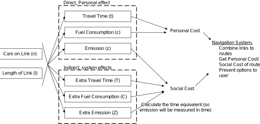
This chapter describes how social navigation works. The users get information about their travel time, and the increase in travel time of other drivers. This might persuade drivers to help others which will increase the networks efficiency. The chapter also describes how the system gets this personal/social information?
When Peter plans his route his navigation system will connect to a server hosting social navigation by using the internet. The navigation system will then request the estimated travel time, and social cost of driving a certain stretch of highway at time t. So now the navigation system gets an up-to-date travel time and social cost estimation instead of having its own database of estimated travel times for all the parts of the network. Social cost, in this setting, represents the time loss for other drivers when driving a stretch of highway. Social cost occurs when driving a link will slow other drivers down, which is nearly always. Because social cost signifies the time loss for others and personal cost
signifies individual travel time, minimizing the sum of personal- and social cost will minimize the total time traveled.
However, since time isn’t all that matters in the social cost, this research also includes increased fuel consumption and emission of other drivers. Accordingly, the social cost is the aggregation of all indirect negative effects a driver causes when driving a link. In this research the social cost will be demonstrated using travel time loss for other drivers (T), extra fuel consumption of other drivers (C) and CO2 Emission (z & Z). In further research this can easily be extended with for example, safety,
comfort, particulate matter emission and/or NOx emission using the framework presented here.
Cars on Link (n)
Length of Link (l)
Extra Travel Time (T) Emission (z) Fuel Consumption (c)
Travel Time (t)
Extra Emission (Z) Extra Fuel Consumption (C) Direct, Personal effect
Indirect, system effects
Personal Cost
Social Cost
Navigation System,
Combine links to
routes
Get Personal Cost/
Social Cost of route
Present options to
user
Calculate the time equivalent (so emission will be measured in time)
[image:7.595.76.528.386.603.2]Figure 1: The framework: calculation of the Personal- and Social Cost by the server
Figure 1 gives a schematic overview of the inner workings of the server. The server first estimates the effects on emission, fuel cost and travel time and then combines them into personal and social cost. Personal cost is everything a driver would normally take into account when driving such as, travel time and fuel consumption cost. Social cost is the “time” loss for other drivers when driving a link.
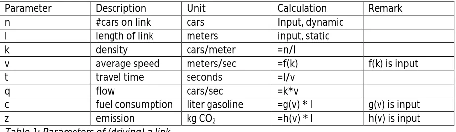
Parameter Description Unit Calculation Remark n #cars on link cars Input, dynamic
l length of link meters input, static
k density cars/meter =n/l
v average speed meters/sec =f(k) f(k) is input t travel time seconds =l/v
q flow cars/sec =k*v
c fuel consumption liter gasoline =g(v) * l g(v) is input z emission kg CO2 =h(v) * l h(v) is input
Table 1: Parameters of (driving) a link
Capital letters of these parameters denote the indirect effect, e.g. the effect a driver has on other drivers. These definitions allow all the personal and social link costs to be expressed in terms of n and l and the three functions. The various costs per link are as shown in table 2. All derivatives are
derivatives to k. For the detailed derivation see appendix 1.
t = l/(f(k))
= ∗ 1
( ) ∗
c = g(v) * l = ( ) ∗
[image:8.595.66.528.83.217.2]z = h(v) * l = ℎ( ( ))′ ∗
Table 2: Various costs per link.
For f(k), h(v) and g(v) the following suggestions are made, these are just examples and can be improved with further research.
f(k) could be a solution of = after substituting q = k*v. This formula is often used to
estimate speed and travel time. A research which contains an overview of many of these speed/flow relationships (and thus potential f(k) function) has been done by Skaberdonis & Dowling.
h(v) could be a transformation version of the formula described in Barth & Boriboonsomin, 2008:
/ = ∗ ∗ ∗ ∗ which describes the real world emission as a function of the non-steady state speed. A related transformation used in chapter 3 is shown in appendix 4.
g(v) can be a simple constant times h(v). Since the chemical composition of fuel is known the amount of CO2 can be calculated. Suggested conversion is 1 liter fuel = 2.4kg CO2 see appendix 2 for
more information.
To obtain the personal and social cost the server now converts all costs described above to seconds using the following rules:
1 second equals 1 second
1 kg of CO2 emission equals 7 seconds
1 liter of fuel (just the cost of it) equals 180 seconds.
There are a few limitations to the inner workings of social navigation so far.
n is an estimated value and therefore has uncertainty
Traffic flow is assumed homogenous on links
No interaction between links has been taken into account, increasing social cost on one might, in reality, decrease traffic on another.
Multiple vehicles problem: Two cars not driving a link doesn’t equal two times one car not driving a link. See description further on this problem below.
All vehicles are assumed equal in emission and number of passengers
The first four points can be solved. Let’s start with the uncertainty in n. This is solved by not using a single value for n in the formulas above, but use a normal distributed variable for n. This will result in a distribution for the personal and social cost. The average of this is a good estimate of the personal and social cost. This average will most likely be higher when using a normal distribution for n, as both personal and social cost functions are convex.
The good thing is, the approach used above solves three of the other problems as well. Inhomogeneous flow can be “simulated” by inserting a variance into the density, which equals inserting a variance into the number of vehicles (since k*l=n). Another option to solve this limitation is by simple splitting a link with length l into many small parts and then applying the formulas to every part. No interaction between links is simply an uncertainty in the estimation of the number of vehicles, thus a variance again. The multiple vehicle problem is solved as well, when 10 cars don’t drive a link they should have the savings of 10 cars which are not driving the link divided by 10. 10 cars not driving should save more than 1 car not driving and thus assuming a variance in n again is a good option.
Since the uncertainties of the problems above are likely to be independent adding the variances is easy.
The last point which assumes that all vehicles are equal remains a problem which is hard to solve. A car with 3 passengers gets equal priority as a 1 passenger car, even though the car with 3 passengers should be 3 times as important when travel time is concerned.
Now the whole system of social navigation is described. To summarize, the server will work as follows. The server in turn
1. Has the static information for l, f(k),g(v) and h(v) for every link (l differs per link, the formula’s are the same for global effects).
2. Computes, personal and social cost for many realistic values of n and σ and stores them into a database1
3. Receive n and σ dynamically from the internet2 .
4. When requested by a navigation system the server responds with the personal and social cost of a link by looking in the database for the closest approximation of n and σ.
Theoretically this process in combination with an optimal altruism level will shift the road system from Nash equilibrium towards the social optimum, from Wardrops user equilibrium towards the system optimum.
This chapter has now provided answer to the first research question. Combining the different impact is done here and a framework for social navigation has been made.
1 Storing the results for all possible number of vehicles and variances won’t result in a big database but will
greatly reduce computational load.
Costs of driving
(20m/s)
Fuel (15%)
Emission (2%)
Time (83%)
Having answered the questions above the second research question is also answered. A car driving at 20 m/s (70 km/h, 45mph) emits around 3 grams of CO2 and uses around 1 milliliter of fuel (appendix
4). This results in the following social costs transformed to time (appendix 2) are: 1 second of time, 0,021 seconds of CO2 and 0,81 seconds of fuel cost.
So when optimizing the system, emission doesn’t really matter as it’s less than 2% of the total social cost. Figure 2 shows the costs of driving.
Aside from the low impact of emission, it’s likely that there is a high correlation between travel time and fuel consumption and emission. These two reasons lead to the conclusion that the social optimum is mainly about optimizing travel time, and the impact of emission is negligible.
[image:10.595.316.519.128.347.2]The next chapter will develop a micro-simulation model to test if the algorithm described above works and will answer the third and final research questions.
3 System Evaluation
This Chapter will answer the final research question by finding the effects of social navigation under different circumstances. First the simulation setup will be described, and then the results will be analysed.
3.1 Simulation setup
To obtain the results, a newly developed micro-simulation model called VBSim was used. VBSim is programmed using visual basic and simulates the behavior of the individual cars based on research of Gipps (1981, 1986). The cars drive through the network to represent a real life situation, allowing social navigation to be tested. The basics of the model and its assumptions are described in appendix 3.
Social Navigation has been implemented as described in chapter two, with a few differences. Instead
of the formula described in chapter two the social time cost of a link will be estimated by the extra time it takes to travel a link because of congestion: tcurrent-tfreeflow. This is a good approximation for
simulation purposes as described in appendix 4. Another difference is that fuel cost is not included in the personal cost as it is expected that people drive solemnly to minimize their travel time.
Emission is based on the formula described in Barth & Boriboonsomin, 2008, after a convertion as
described in appendix 4 this results in a formula which gives the emission per second based on speed.
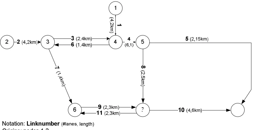
The network is loosely based on the bay area. It contains three bridges which will be bottlenecks as
[image:11.595.72.491.481.696.2]traffic increases. The western bridge (#7) is for many drivers the shortest way, and will therefore be congested first. The middle bridge (#8) is the second best alternative and will congest second. The eastern bridge (#5) will not congest, but is very long. A simplification of the network is shown below in figure 3. This network has been chosen because it has different links with different levels of congestion.
3.2 The Results
To obtain the results a default run is set up. To answer the research questions a certain aspect of the default run will be changed. The default run assumes high traffic, so that link 7 congests and link 8 experiences a slight travel time increase: 1300 cars/hour from node 1 to 6, 1 to 8, 2 to 6 and 2 to 8 for a total of 5200 cars/hour entering the network. Furthermore it is assumed that 20% of the drivers are regular drivers which listen to the radio and therefore behave as if they use “dynamic navigation” and that 20% of the drivers have a dynamic navigation system and 20% of the drivers have a social navigation system. So 20% drives socially, 40% drives dynamically and 40% drives static. It is assumed that the average driver is willing to sacrifice 1 minute of his own if this saves other drivers at least 4 minutes.
After 6000 seconds the total social cost is divided by the number of cars which entered the network. This approximates the average travel time for drivers. But also includes the social aspects such as fuel consumption and CO2 emission weighted as described in appendix 2.
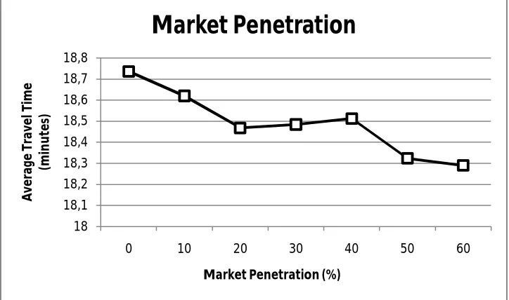
Market penetration
[image:12.595.72.434.386.600.2]To study the effect of the percentage of drivers using social navigation 210 simulations of 6000 seconds were done. The simulations are done with social navigation levels of 0 to 60% of the total numbers of drivers equipped with social navigation. To compare social navigation with dynamic navigation at all time 60% of the drivers use either social- or dynamic navigation so if 10% drives socially then 50% drives dynamically. The results varied highly per run, which is why there were so many runs done. The results can be seen in the graph, figure 4.
Figure 4: The effects of market penetration on travel time
As can be seen, higher levers of market penetration result in lower social cost per car. A student-t tests between the results of market penetration 0% and 60% shows that the probability that social navigation does not decrease travel time compared to dynamic navigation of 2,7E-05 which means that there is no doubt that social navigation indeed helps. The results may not seem large (i.e. ½ minute per car), but with an average of 5200 cars per hour that means about 45 hour can be saved every hour in the simulated network. In other words, saving ½ minute on an 18.5 minute trip saves the average driver 2.7% on their time.
18 18,1 18,2 18,3 18,4 18,5 18,6 18,7 18,8
0 10 20 30 40 50 60
A ve ra ge T ra ve l T im e (m in u te s)
Market Penetration (%)
Looking at the graph it seems that the effect of one more social driver on the system is greater when market penetration is low. This however, due to the high variance of the road system, which could not be significantly proven.
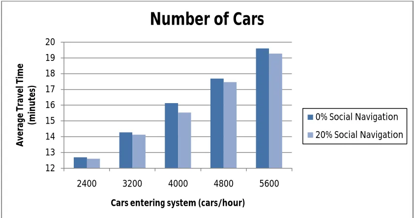
Congestion
[image:13.595.87.509.191.413.2]To test the effect of different congestion levels in the network the simulation has been run with varied number of vehicles in the network. At 2400 vehicles per hour entering the network there was very limited congestion, however when 5600 vehicles per hour enter the network even link 8 was congested.
Figure 5: the effect of the number of cars on the effect of social navigation
As is to be expected, and the graph shows, the effects of social navigation increase as congestion increases. This is due to the fact that with few cars on a link, driving that link won’t increase the congestion and therefore there is no social cost. This conclusion proves significant.
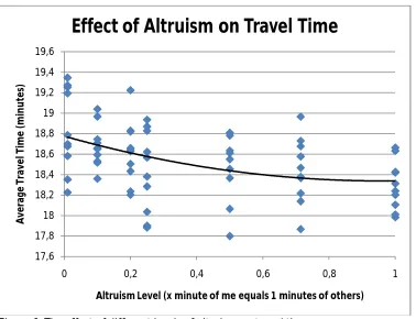
Altruism
To test the effects of different levels of altruism the following approach has been used. It has been assumed that every driver using social navigation values 1 minute of his own equal to x minutes of someone else. So if x = 0 the drivers don’t care about others (which therefore equals dynamic driving), if x = 1 the drivers value other just as much as they do themselves (best case). So higher values of x represent more altruistic behavior.
12 13 14 15 16 17 18 19 20
2400 3200 4000 4800 5600
A
ve
ra
ge
T
ra
ve
l T
im
e
(m
in
u
te
s)
Cars entering system (cars/hour)
Number of Cars
0% Social Navigation
Figure 6: The effect of different levels of altruism on travel time.
As can be seen in the graph, and is statistically significant, social cost tends to improve as drivers behave more altruistic. It could be expected that altruism is more important at lower levels of altruism. This because accepting to save 80 minutes sacrificing 3 minutes will benefit the system more than saving 5 minutes sacrificing 3 minutes. This also looks to be the case when looking at the best-fit second order polynomial. Based on the data this seemed probable but was not statistically significant.
17,6 17,8 18 18,2 18,4 18,6 18,8 19 19,2 19,4 19,6
0 0,2 0,4 0,6 0,8 1
A
ve
ra
ge
T
ra
ve
l T
im
e
(
m
in
u
te
s)
Altruism Level (x minute of me equals 1 minutes of others)
4. Conclusions
This research designed social navigation and tests this using a newly developed micro-simulation model. The tests were carried out under varying levels of altruism traffic intensity and market penetration. Social navigation is an addition to dynamic navigation; it does not only use real-time traffic information but also allows drivers to help each other.
To evaluate different impacts of social navigation CO2 emission, travel time and fuel cost have been
combined into one overall value. This was based on various pieces in literature, but due to disagreement in literature an estimation has been made. This combination has then been used to build the framework of social navigation. This framework is adaptable because it relies on function which can still be defined. The choice of these functions determines the workings of the social navigation. For these functions examples have been given with reference to literature. Finally, social navigation has been tested by developing a micro-simulation model. The micro-simulation uses Gipps car following model (Gipps, 1981) and Gipps lane-changing (Gipps, 1986). The network simulated is loosely based on the bay area, it has two origins two destinations and three alternative routes which overlap from time to time. Traffic is assumed to be high. The emission in the model was estimated as described by Barth & Boriboonsomin (2008). Other assumptions were described in appendix 3, 4 and 5. These either reduce the efficiency of social navigation, or are of limited impact on social
navigation.
The results compare dynamic navigation to social navigation under different circumstances. Because of the high variance of the road system many simulations have been done. The findings are that social navigation works better (i) at higher market penetrations, (ii) when there is more congestion and (iii) drivers behave more altuistic. All these results are statistically significant. Social navigation saved up to 2.5% more travel time than dynamic navigation in the simulated network. When
implemented on a large scale and more people driving altuistic the economic benefits is expected to be very high.
Social navigation not only optimizes travel time but also emission and fuel consumption. So the 2.5% travel time reductionactually represents a 2.5% social cost reduction. Interesting, however is that social navigation doesn’t result in emission reduction and sometimes even results in a slight emission increase. This is because the impact of emission on society is much lower than time loss. Social navigation therefore mainly decreases travel time.
4.1 Further Research
This research explored the basic possibilities of social navigation and designed a framework which is flexible. This creates the opportunity for various kind of further research. A few possibilities are listed hereafter.
Add more factors. Currently the research includes CO2 emission, fuel cost and travel time.
Other factors like particulate matter emission, reliability, safety, comfort and/or equal share of recourses could be added.
Filling up the framework: This research presents a framework for social navigation. Further research could study the formula’s used as input for this framework and perhaps include hills in the emission formula.
accurate real-time information and offering other incentives beside altruism to use the system.
References
Anthoff, D., Hepburn, C., & Tol, R. S. (2008). Equity Weighting and the marginal damage cost of climate change. Ecological Economics .
Barth, M., & Boriboonsomin, K. (2008). Real-Word CO2 Impacts of Traffic Congestion. Transportation
Research Board .
Brackstone, M., & McDonald, M. (1999). Car-following: a historical review. Transportation Research
Part F 2 , 181-196.
Clarkson, R., & Deyes, K. (2002). Estimating the Social Cost of Carbon Emissions. Department of Environment, Food and Rural Affairs, Environment Protection Economics Division, London.
DeNavas-Walt, C., Proctor, B. D., & Smith, J. C. (2008). Income, Poverty, and Health Insurance
Coverage in the United States 2007. Washington D.C.: USCensusBureau.
Gipps, P. (1981). A Behavioural Car-Following Model for Computer Simulation. Transportation
Research Board 15B , 105-111.
Gipps, P. (1986). A Model for the Structure of Lane Changing Decisions. Transportation Research
Board 20B , 403-414.
Hope, C. (2008). Discount rates, equity weights and the social cost of carbon. Energy Economics 30 , 1011-1019.
Pearce, D. W. (2003). The Social Cost of Carbon and its Policy Implications. Oxford Review of
Economic Policy, Vol. 19, No. 3 , 362-384.
Rakha, H., Pecker, C. C., & Cybus, H. B. (2007). Calibration Procedure for Gipps Car-Following Model.
Transportation Research Record 1999 , 115-127.
Skaberdonis, A., & Dowling, R. (n.d.). Improved Speed-Flow Relationships for Planning Applications.
Transportation Research Record , 18-23.
Walters, A. A. (1961). The Theory of Measurement of Private and Social Cost of Highway Congestion.
Appendix 1.1 – calculating T
=
( )= f(k) = v by definition
∆
( ) =∆
( ) ∗ ∆ =∆ Approximation
( ) ∗ ∆ ∗ =∆ ∗ = = time/car*cars = time
( ) ∗ ∆ ∗ ∗ = k = n/l
∗ ( ) ∗ ∆ ∗ ∗ = constants can be taken out of the derivative
( ) ∗ ∗ ∗ ∆ = L/L=1
∗ ( ) ∗ = Δn = 1 (1 vehicle enters the link)
An intuitive explanation of this formula is: change in travel time (1/speed, 1/f(k)) times the number of cars effected (k*l) equals total time lost.
Appendix 1.2 – Calculating C and Z
For derivation of C just substitute g(v) for h(v)
h(v) = amount of CO2 emitted per meter as a function of speed.
f(k) = speed as a function of density
∗ ℎ( ) = ∗ ∆ℎ( ) = ∆
∗ ℎ( ) ∗ ∆ =∆
∗ ℎ( )′ ∗ ∆ ( ) =∆
∗ ℎ( ) ∗ ( ) ∗ ∆ =∆
∗ ℎ( )′ ∗ ( ) ∗ ∆ =∆
∗ ℎ( ) ∗ ( ) ∗∆ =∆
∗ ℎ( ) ∗ ( ) ∗∆ ∗( ) =∆ ∗ = ℎ =
∗ ℎ( ) ∗ ( ) ∗1∗( ∗ ) =
chain rule
∗ ℎ ( ) ∗ = Z
Appendix 2 - Combining the Values
Conclusion
1 kg CO2 = $0.04 (1)
$0.04 = 1/500 carhour (2) = 7 sec
1 liter fuel = 1/3.79 gallon (6) 1/3.79 gallon = $1 (4) $1 = 1/20 carhour (2) =180 sec
1 liter fuel = 0.75kg fuel (5)
= 2.4kg CO2 (3)
1: 1kg CO2 = $ 0.04 (year 2008 dollar)
Various researches about the social cost of carbon have been conducted. In a research for the British government Clarkson & Deyes (2002) concluded the appropriate social cost was about $100 (year 2000 dollars) per ton Carbon. In response to this report, Pearce (2003) conducted a study of his own. He concluded that the estimate by Clarkson & Deyes was far too high and argued that the right value was between $5 and $27 per ton Carbon. The two most recent researches are from Hope (2008) and Anthoff et al. (2008). Both review the researches from Clarkson & Deyes and Pearce and describe the different approaches for obtaining the social cost of carbon. Both researches result in a very high uncertainty estimate with lows around $7/tC and highs of $2500/tC. Hope expects a value of around $69 and Anthoff estimates the social cost $200/tC.
A choice for the social value is hard to make. In this research a value of $100/tC (year 2000) will be used. This value is above the value of Pearce and the value of Hope, and below the value of Clarkson & Deyes, and the value of Anthoff et al. After applying a 4% interest rate, changing from C to CO2
(1kg C = 44/12 CO2) this results in approximately $40 per 1000kg CO2
A different option not adopted for estimating the cost of emission is the use of Carbon Credits. Carbon Credits exist because the government limits the amount of emission of a certain
company/branch. Emitting less than your allowance allows you to sell your unused credits, emitting more will force you to buy these credits. This way the emission gets a value and theoretically this will result in saving emission where it is the cheapest. This works since CO2 is a global problem and it
therefore doesn’t matter where the savings happen. Currently the biggest implementation of Carbon Credits is the European Union Emission Trading Scheme. The price for a Carbon Credit (1 ton of CO2)
equals 22 euro3 ($0.033 per kg CO2). This cost however is of limited use for this research as this
represents the cost to reduce pollution instead of the effect of pollution. The price of a Carbon Credit depends highly on the limit of emission determined by the government and this way has limited relation to the impact of emission. Therefore the social costs found in the literature as described above best suited for this research.
2: 1 carhour = $20 (year 2008)
The ‘cost’ of the time lost when driving used in this research should equal the willingness of a certain person to pay for saving this time. This however is impossible to measure because this differs from
3
one person to another and differs for the number of passengers in the car. The research will therefore assume 1 value for every car.
The median income in 2008 for someone working full-time is about $32.000 (DeNavas-Walt, Proctor, & Smith, 2008), average working hours is 1750, OECD(2004)4. This results in a net income of around $18 per hour. Taking into account an average number of people per car which is greater than 1 and people liking sitting in the car about equal to being at work, the estimate of $20/carhour is taken.
3: 1 kg of fuel = 3.2 kg CO2
Gazoline is about 87% C by weight5. Since 1 mole of C will result in 1 mole of CO2, and taking into
account the weight of C (12) and O (18) the conclusion follows.
4: 1 Gallon Fuel = $3.7 per gallon6 5: 0.71–0.777 liter fuel = 1 kg
6: 1 US gallon = 3.79 liter
7: 1g CO2 = 12/44g C Chemistry (C=12, O = 18)
4
http://dx.doi.org/10.1787/174615513635
5
http://www.fueleconomy.gov/Feg/co2.shtml
6
http://www.eia.doe.gov/oil_gas/petroleum/data_publications/wrgp/mogas_home_page.html
Appendix 3 - Inner workings of VBSim
The basics
Links:
number of lanes
speedlimit
Lanes
Vehicles drive on lanes
11 signifies link 1, left lane. 73 is link 7 lane 3rd (from the left)
Node
Nodes are stored as an array, connect. Connect(lanenumber1) results in lanenumber2, where the lanenumber1 continues, or a 0 if the lane ends.
Cars
Lanenumber, the lane on which the car drives
Position, the distance to the start of the lane (integer value in meters)
speed, the speed of the car (integer value in meters/second)
CarinFront, the car which is in front of this car
CarBehind, the car which is behind this car
Destination, the final destination of the car
Targetlane, the lane the car wants to go in order to reach the final destination
Type, shortest route, dynamic route or social route
The simulation steps
Steps are 1 second, the following parameters are updated.
Cars entering the network,
For every lane there is a x/3600 % chance that a vehicle will be spawned. Where x is the number of vehicles starting from that lane per hour.
The car starts with a speed which equals the longitudal behavior described below (vcomfort=
∞
)Longitudal Behavior
The speed is the minimum of comfortspeed, safespeed and nodespeed
( + 1) = min ( + 1), ( + 1), ( + 1)
Safespeed is the safe speed which makes sure that the car doesn’t hit the car in front. This is based on Gipps (1981), willingness to brake is assumed -3m/s2 and reaction time 1 second. Gipps formula is a simple derivative from basic mechanics assuming that the car in front might decelerate with -3m/s2.
( + 1) = −3 + 9 + 3(2( −1)− ( ) + ( ) 3
v = speed of the car
v^= speed of the car in front x = distance between cars
Length of a car is assumed 4 meters
Comfortspeed is the speed which makes sure that the car accelerates/decelerates smoothly. This is again based on Gipps.
( + 1) = ( ) + 7.5∗ 1− ( ) ∗ 0.025 + ( )
vmax = speedlimit
Nodespeed is the speed which makes sure that the car decelerates when it’s getting near a node and isn’t in the right lane. If the car is in the wrong lane, the speed is limited in the same way as done with safespeed. The node is assumed to be a stationary object (v^=0).
Lane-Changing Behavior
Lane changing will be based on Gipps (1986). After some simplifications VBSim will work as follows:
1. Is there a lane to go to?
Is there a lane to my left/right? 2. Is there a gap for me to fit in?
a. How hard should I brake to avoid the driver who would be in front of me? b. How hard should the driver who would be behind me brake?
3. How much do I want to fit in the gap?
a. Is there a turn I should take close (if <10 sec, willingness to break doubles according to Gipps)
b. Is there a speed advantage (when speed advantage passes a threshold driver will try to switch lanes with willingness to brake -3m/s2)
4. If the willingness to brake (3) is larger than the necessity to brake (2), change lane
Route-choice
To determine if a car is in the right lane Dijkstra’s shortest path algorithm is used. Depending on the type of driver (static/dynamic/social) different weight for the edges are used.
Limitations/assumptions:
No direct calibration has been done. The model has not been calibrated using real-life data. This isn’t a big problem as various pieces of literature describe the accuracy of the formula’s of Gipps, which serves the purpose as it’s main limitation is that it only considers one car ahead (Brackstone & McDonald, 1999 and Rakha, Pecker, & Cybus, 2007)
Only one network has been tested.
Cars nearing an exit (closer than 50 seconds) will not change lanes to increase their speed.
Drivers only take the shortest route. In reality drivers often take the second shortest route.
No hills, accidents, road work and weather conditions have been taken into account. This is no big limitation as this dynamic changing of the road system will only increase the efficiency of dynamic and social navigation,
The model uses integer values only, for time as well as distance. This might result in rounding errors, but the impact will probably be low.
Because Gipps speed function isn’t influenced by the lane changing it sometimes happen that two vehicles in adjacent lanes want to change lanes. But because they have equal speed and because their exit is equally near they’ll decelerate equally fast. This will result in the two vehicles coming to a stop near the exit because neither can switch lanes. This has been solved by switching the cars when this problem arises. While this isn’t realistic it shouldn’t affect macro effects of the simulations too much. This switching happens on average once every 5 seconds.
Appendix 4 – Converting the emission formula
/ = ∗ ∗ ∗ ∗ (Barth & Boriboonsomin, 2008)
This formula is modified to gram CO2/s by the following steps:
1. Both sides times mph, result:
ℎ = ℎ ∗
∗ ∗ ∗ ∗
2. Substitute every mph by (2,2369362921 * m/s)
3. Convert hour to seconds by dividing both sides by 3600
4. Merge the constant which appears on the right hand side of the equation with b0 by taking
it’s natural logarithm and adding it to b0
5.
To check if no errors were made a simple check is performed. A car drives 20 m/s
A car drives 15 km/liter = 15000 m/liter A car drives 1/750 liter/sec
1 liter = 2.4 kg CO2 (see appendix X)
so a car drives 2.4kg/750sec so a car drives 3.2 gram CO2/sec.
This is in the same range as the graph produced earlier which indicates that there weren’t made any mistakes in the process.
0 2 4 6 8 10 12 14 16 18
0 5 10 15 20 25 30 35 40
Em
is
si
o
n
(g
ra
m
C
O
2
/
s
e
c)
Speed (m/s)
Appendix 5 - Calculating the Social Time Cost
The social time cost (T) of a link is the total time cars lose when 1 additional car drives the highway.
This will be calculated by making the following simplification of a piece of highway (see figure). The time loss in this figure equals the number of vehicles waiting to exit times the time a vehicle takes to exit (i.e. nc * 1/q).
lu length of the uncongested part meters
lc length of the congested part meters
lt total length of the link meters
vu average speed at the uncongested part meters/second
vc average speed at the congested part meters/second
tu travel time of the uncongested part seconds
tc travel time of the congested part seconds
tt total travel time of the link seconds
nc total number of cars in the congested part cars
kc the density of cars in the congested part cars/meter
q total outflow of cars of the link (cars/second) cars/second
T Time Loss Seconds
assumption: 0 ≤vc<vu≤vm asdk v
Part 1
= + Follows from definition
= + t = l/v
= + Follows from definition
= + lu = lt-lc (see last line)
= − + Split quotient
− = − tfree = time it takes the lane when uncongested = lt/vu
∆ = − Δt = t-tfree
Part 2
= ∗ because k=n/l
= ∗ because k*v=q
= ∆ ∗ Using the result of part 1
Part 3
= ∗ Time lost = (Cars in queue) * (Time it takes to for 1 car to leave the queue)
= ∆ using result of part 2
= By definition vc<vu
≤ ∆
vc/vu is probably very small. Therefore the following approximation is taken as a function for the social time cost in VBSIM:
=∆ = −
This is an underestimation of social time cost because:
Doesn’t account for time loss in the uncongested part (which might be significant)
vc/vu > 0
This underestimation results in an underestimation of the effects of social navigation. Assume that the real social cost is x% higher. Since the social cost is divided by the level of altruism