On an Adaptive Filter based on Simultaneous Perturbation Stochastic Approximation Method

On an Adaptive Filter based on Simultaneous

Perturbation Stochastic Approximation Method

Hong Son Hoang, R´emy Baraille

Abstract—In this paper, the simultaneous perturbation stochastic approximation (SPSA) algorithm is used for seeking optimal parameters in an adaptive filter developed for assimi-lating observations in very high dimensional dynamical systems. It is shown that the SPSA can achieve high performance similar to that produced by classical optimization algorithms, with better performance for non-linear filtering problems as more and more observations are assimilated. The advantage of the SPSA is that at each iteration it requires only two measurements of the objective function to approximate the gradient vector regardless of dimension of the control vector. This technique of-fers promising perspectives for future developement of optimal assimilation systems encountered in the field of data assimilation in meteorology and oceanography.

Index Terms—adaptive filter, minimum prediction error, Schur vector, stability, stochastic approximation

I. INTRODUCTION

D

ATA assimilation is a technique of (optimally) com-bining numerical model with observations. Let us first consider the standard 4dVar assimilation algorithm which is formulated as follows [1]: Find the initial statex(0) :=x(t₀)

which minimizes the objective function

J[x(0)] = (1/2)(xb(0)−x(0))TB(0)−1(xb(0)−x(0)) (1)

+(1/2)N_k=1[z(k)−Hx(k)]TR−1[z(k)−Hx(k)]

under the constraint

x(k+ 1) = Φx(k) +w(k), k= 0, ... (2)

z(k) =Hx(k) +(k), k = 1, ... (3)

herex(k)is then-dimensional system state at k:=t_k,Φ is the (nxn) fundamental matrix,z(k)is the p-dimensional observation vector, H is the (pxn) observation matrix, w,

are the model and observation noises. We assumew(k), (k)

are uncorrelated sequences of zero mean and time-invariant covarianceQandR respectively.

Applying a gradient descent algorithm, at each iteration the gradient ∇_θJ, θ := x(0) is used to determine the direction to searchJ_min. The gradient computation requires a forward integration of the numerical model over the period

[t₁, t_N] and backward integration of the adjoint ΦT of Φ. The development of a discrete adjoint solver for partial differential equations by hand differentiation requires a long development time and it involves the errors resulting from necessary approximations used during the differentiation.

Manuscript received March 23 2011; revised April 06 2011.

H.S. Hoang is with the Service Hydrographique et Ocanographique de la Marine (SHOM), 42 av Gaspard Coriolis 31057 TOULOUSE FRANCE, emails: [email protected].

R´emy Baraille is with the Service Hydrographique et Ocanographique de la Marine (SHOM), 42 av Gaspard Coriolis 31057 TOULOUSE FRANCE, Email: [email protected]

Another approach for data assimilation is known as se-quential. Consider (3) and the interval [t_k−1, t_k]. Then z= z(k) and xˆ(k/k−1) := xb(k) represents the predicted estimate forx(k). Taking the derivative ofJ(θ)and equal it to zero leads to the equation for finding the optimal filtered (or analysis) estimatexˆ(k). One has now

ˆ

x(k) = ˆx(k/k−1) +K(k)[z(k)−Hxˆ(k/k−1)] (4)

K(k) =B(k)HT[HB(k)HT +R]−1 (5) in which K(k) represents the filter gain, ζ(k) = z(k)− Hxˆ(k/k −1) is the innovation vector, B(k) := M(k)

represents the covariance of the prediction error (PE)e(k/k− 1) := ˆx(k/k−1)−x(k). The unbiased minimum variance (MV) estimate for x(k) is obtained from the Kalman filter (KF) (see [2]). The closed system of equations for the KF includes Algebraic Riccati Equation (ARE). However solving the ARE for the system with state dimensions1012−1014 is impossible.

To deal with these difficulties in [3] the filter is assumed to be of the form (4) with the gain K(k) :=K(k;θ) being given up to a vector of unknown parametersθ. The optimal filter is obtained by minimizing the prediction error (PE) for the system output

J(θ) =E[Ψ(ζ(k))]→minθ,Ψ[ζ(k)] =||ζ(k)||2 (6)

where ||.|| denotes the l₂ norm. As the use of estimated parametersθˆ(k)can deviate the filter from its stable behavior, in [5]-[6] the gain is proposed to be selected in order to ensure a filter stability, independently on whatever are the values of tuning gain parameters.

The purpose of this paper is to explore what potential benefits may be achieved by using SPSA algorithm [8]. The essential feature of SPSA is its underlying gradient approximation that requires only two measurements of ob-jective function regardless of the dimension ofθ. This feature allows for a significant decrease of the cost of optimization, especially without development of the adjoint code for the tangent linear model (TLM) of the system dynamics.

II. SPSAALGORITHM

A. Stochastic approximation [4]

Consider the problem of minimizing the objective function

Find θ∗that solvesmin_θJ(θ) (7) For an unconstrained optimization, many iterative algo-rithms rely on the gradient vector g(.) of the objective

function. The stochastic approximation (SA) algorithm has the form

θ_k+1=θ_k−a_kY(θ_k) (8)

where Y_k = g(θ_k) +noise, a_k is a non-negative gain sequence that must satisfy certain conditions [8].

When only the measurements of the objective function are available, y_k =J(θ_k) +noise, one-sided or two-sided gradient approximations, i.e.g_ki(θ_k) = y(θk+ckei)−y(θk)

ck or

g_ki(θ_k) = y(θk+ckei)−y(θk−ckei)

2ck are of common use where

e_i denotes a vector with a one in the ith place and zeros elsewhere. These approximations requiren_θ+1(or2n_θ,n_θis the dimension ofθ) integrations of the numerical model. For optimization problems with very large n_θ, such algorithms are expensive and in general they are inappropriate for solving assimilation problems.

B. Simultaneous Perturbation Stochastic Approximation (SPSA)

The difficulties due to high dimension of θ can be over-come by applying the SPSA algorithm [8]. In such algorithm, all elements ofθ_k are randomly perturbed together to obtain two measurements y(.), but each component of g_k(θ_k) is formed from a ratio involving the individual components in the perturbation vector and the difference in the two corresponding measurements. For two-sided SP, we have

g_ki(θ_k) = y(θk+ckΔk)−y(θk−ckΔk)

2ckΔki whereΔkican be chosen as the random variable having the symmetric Bernoulli (+/-) 1 distribution. Two common distributions that do not satisfy the conditions forΔ_ki are the uniform and the normal.

III. ADAPTIVE FILTER A. Adaptive filter

Consider the KF (4)(5) for solving a filtering problem in the system (2)(3). ThenB(k) :=M(k) satisfies the Riccati equation

M(k) = Φ(k)P(k−1)ΦT(k)+Q, P(k) = [I−K(k)H]M(k)

(9) Due to very expensive computational burden in time stepping the prediction error covariance matrix (ECM)M(k)

in (9), the KF is impractical for solving data assimilation problems. For suboptimal KFs for data assimilation, see [1],[9]. One of possible ways to overcome these difficulties is to choose a parametrized structure of the filter gain from some criteria. In [5] this question is studied from the point of view of the filter stability. The following time-invariant structure of the gain is proposed

K=P_rΘK_e, K_e=H_eT[H_eH_eT+R]−1, H_e=HP_r, (10)

Θ = diag[θ₁, ..., θ_ne], θ_l∈(0,2)

whereK_e : Rp →Rne _{represents the gain mapping the} innovation vector from the observational space into the reduced space Rne _{of dimension ne} ≤ _{n; Pr is mapping} from the reduced spaceRne_{to the full spaceR}n_{. The choice} of the reduced space plays an important role in assuring a

stability of the filter. As proved in [5], under detectability condition, stability of the filter is ensured by forming the columns of P_r from a subspace spanned by leading eigenvectors (or Schur vectors) of the fundamental matrix

Φ. The AF is obtained by minimizing the objective function (6). In the AF the gain Kin (9) becomes time-varying.

IV. NUMERICAL PROCEDURE FOR CONSTRUCTION OF THE PROJECTION SUBSPACE

A. Computation of projection subspace spanned by leading Schur vectors [10]

The idea for construction ofP_rbased on stability criteria is outlined as follows. LetLbe an integer number satisfying

1 ≤ L ≤ n. Given an n×L matrix X₀ with orthonormal columns, the method of orthogonal iteration generates the sequence of matrices X_i,

S_i= ΦX_i−1, X_iG_i=S_i, i= 1,2, ...,

whereX_i is orthonormal. Thus, atiiteration, the columns of X_i are orthonormal vectors which are derived by : 1) integration of the model from each column of X_i−1 to produceS_i; 2) orthonormalization ofL columns ofS_i. One sees that the columns of S_i belong to the space spanned by the vectors ofX_i.

Let

XTΦX =T =diag(λ_i)+ ¯N ,|λ₁| ≥ |λ₂| ≥...≥ |λ_n| (11)

be a real Schur decomposition, X = [X1, X2], X1 is

n×Lsubmatrix,N¯ is a block upper triangular. The blocks on the diagonal of N¯ are of size 1x1 (in which case they represent real eigenvalues) or 2x2 (in which case they are derived from complex conjugate eigenvalue pairs). As shown in [10] (section 7.3), under mild conditions, the distance between D_L(Φ) := R[X1] and R[X_i] is of order

O(|λL+1 λL |

i_{) where R[Xi] denotes the linear space spanned}

by the columns of X_i. Considering the columns of X_i as patterns for DScVs, the orthogonal iteration method allows us to generate patterns for DScVs which can be used to perform the operatorP_r. This method constitutes a basis of the procedure described in the next subsection for generating PE samples which serve as a source for estimating the statistics of PE and to approximate the filter gain (called a PEF - Prediction Error Filter).

B. Procedure for generating dominant prediction error (DPE) samples

Suppose that at the moment i:=t_i we are givenx_f(i) -some estimate for the true system state x(i). The estimation error is δx(i) = x_f(i)−x(i). Integration of the model from x_f(i) produces the prediction x_p(i+ 1) = Φx_f(i) at

t_i+1=t_i+δt. HereΦrepresents model integration over the intervalδt. The true system state att_i+1isx(i+ 1) = Φx(i)

(for no model error case). We have then the PE e_p(i+ 1) = Φx_f(i)−Φx(i) = Φδx(i). Thus integrating δx(i) by the model Φ yields the vector s_t+1 = Φδx(i) which can be

considered as a PE pattern growing over the period of model integration. If we apply this procedure to an ensemble of orthogonal columnsX_i= [δx1(i), ..., δxL(i)]instead of one vector δx(i), the iteration S_i = ΦX_i−1, X_iG_i = S_i, i = 0,1, ... (see section 3.1) will produce the sequence {X_i}

approaching L dominant Schur vectors of Φ. The relation

X_iG_i = S_i guarantees that the columns of S_i belong to the space spanned by the columns of X_i hence they will approach a subspace spanned by DScVs. As the columns ofS_i at the same time represent the PE samples, they will be referred to in the future as DPE patterns(in the DScVs subspace). These columns are thus not the patterns randomly generated as done in the EnBF [11],[12] but selected to be ”representative” (in a DScV subspace) for the PE. These DPE samples will be used in this paper to estimate the elements or parameters of the ECM which plays an essential role in computation of the filter gainK. We summarize this DPESP for generating the ensemble of PE patterns in the

L-dimensional DScVs subspace as follows:

Suppose we want to simulate T patterns for each of the firstLSchur vectors of the system dynamicsΦ. Ati= 0, let

x_f(i)be an initial estimate for x(i). Suppose we are given the orthogonal matrix X_i, X_iTX_i =I_L whose columns are

Lorthonormal perturbationsδxl_f(i), l= 1, ..., L.

Step 1. For i≤T: Letx_f(i) andX_i be given. Integrate the modelL+ 1times for producingx_p(i+ 1) = Φ(x_f(i))

andx_pl(i+ 1) = Φ(x_f(i) +δxl_f(i)), l = 1, ..., L. The new matrixS_i+1(L) := [δx1_p(i+ 1), ..., δxL_p(i+ 1)] is performed whose columns are

δxl_p(i+ 1) = Φ(x_f(i) +δx_fl(i))−Φ(x_f(i)), l= 1, ..., L

Step 2. Apply the Gram-Schmidt orthogonalization pro-cedure (see [10])X_i+1G_i+1 =S_i+1 to S_i+1. The resulting orthonormal perturbations{δxl_f(i+ 1), l= 1, ..., L}are the columns of the matrixX_i+1 = [δx1_f(i+ 1), ..., δxL_f(i+ 1)].

Step 3. Ifi+ 1> T: Stop the procedure. Otherwise set

i:=i+ 1 and go to Step 1 subject to x_f(i+ 1) andX_i+1. Comment 4.1. The DPESP algorithm can be applied to a nonlinear system dynamics whereF(x)stays instead ofΦx

with the modificationΦδx(i)≈F[x(i) +δx(i)]−F[x(i)]. The columns ofX_i then tend to DScVs of the TLM.

V. ESTIMATION OF PARAMETERS IN PERIODIC SIGNALS

A. Numerical model. Assimilation problem

In the observation model

z(t_k) =f(t_k) +(t_k), f(t) = N

i=1

α_icos(ω_it), k= 1, ..., M

(12) let N be given and M > 2N, (t_k) is a sequence of zero mean and variance σ2. The experiment is performed for estimating the parameters α_i, ω_i (see [13]) where (.)

represents the observation error.

Following [13], foru_i(t) :=α_icos(ω_it), we have

d2u_i dt2 =−ω

2

iui, ui(0) =αi,du_dti(0) = 0 (13)

[image:3.595.300.433.31.147.2]

z(t_k) =N_i=1u_i(t_k), k= 1,2, ...

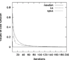
Fig. 1. The values of the objective functions resulting from three algorithms: Newton, SA and SPSA

The vector of unknown parameters θ = (α₁, ..., α_N, ω₁, ..., ω_N) will be estimated by solving the variational problem (for stationary (t_k))

J(θ)→min_θ, J(θ) = 1 M

M

k=1

[z(t_k)−f(t_k;θ))2] (14)

The system (13) can be reformulated in the form equiva-lent to (2)(3) as

dx(t)

dt = 0, x(0) =θ (15)

z(t_k) =h[x(t)] =_iN₌₁α_icos(ω_it), k = 1, ..., M

The task is to estimate the initial system state x(0) by minimizing (14) using the available observations. Comparing (14) with (1) shows that the first term in the right hand side of (1) does not participate in (14) which is equivalent to assuming that there is no a priori information on θ. The observation operator in the present case is non-linear.

B. Numerical results

The true values of the parameters (α_i, ω_i) are that given in [13], i.e. α₁ = 1, α₂ = 0.5, α₃ = 0.1, ω₁ = 1.11, ω₂ = 2.03, ω₃ = 3.42. The corresponding initial values are:

α₁(0) = 0.9, α₂(0) = 0.6, α₃(0) = 0.2;ω₁(0) = 1, ω₂(0) = 2, ω₃(0) = 3; α₁(0) = 0.9, α₂(0) = 0.6, α₃(0) = 0.2.

The measurements are contaminated by the Gaussian noise

N(./m, σ2) with m = 0 and σ2 = 0.01. To estimate θ

we will apply the well known Newton iterative algorithm (see [10]) and two versions of the stochastic optimization algorithm: SA (8) and SPSA (section 1, B).

From Fig. 1 one sees that the objective function, asso-ciated with the Newton-algorithm, decreases most quickly. Compared to the SA, the SPSA-algorithm works better in minimizing the objective function. Globally, all three algo-rithms are capable of well tuning the parameters to decrease the objective function.

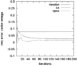
Fig. 2 shows the consistency of three algorithms in esti-matingα. The SPSA-algorithm produces more efficient esti-mate forαcompared to the SA-algorithm. As to the estimates forω, Fig. 3 demonstrates that with noisy measurements, the strategy to fit fast and exactly the output of the model to measurements can lead to big biased estimate as it happens in the Newton-algorithm.

[image:4.595.42.179.37.149.2]

Fig. 2. Consistency of three algorithms in estimatingα

Fig. 3. Estimation errors forωin three algorithms

VI. ALGORITHM OF THEROAFFOR ALTIMETRICSSH DATA ASSIMILATION

A. MICOM model and observations

The Miami Isopycnal Coordinate Ocean Model (MICOM), used here for the twin experiment is identical to that de-scribed in [7]. The model configuration is a domain situated in the North Atlantic from 300 N to 600 N and 800 W to 440W; for the exact model domain and some main features of the oceanic current (mean, variability of the sea surface height (SSH), velocity ...) produced by the model, see [7]. The observations are SSH taken from the control run every 10 days (ds), only at the grid points i_o = 1,11, ...,131,

j_o = 1,11, ...,171 from the grid i = 1,140;j = 1,180. They are noise-free.

B. Reduced-order filter and gain structures

The filter used for assimilating SSH observations is of the form

ˆ

x(k) =F[ˆx(k−1)] +KP_oiζ(k), k = 0,1, ... (16)

where ˆx(k) is the filtered estimate for x(k), x(k) = [h(k), u(k), v(k)]is the system state atk:=t_k,t_k+1−t_k = 10ds,F(.)represents integration of the MICOM nonlinear model over 10ds,Kis the filter gain,ζ(k)is the innovation vector. The operator P_oi will interpolate the missing SSH from observed points. The gainK is symbolically given by

K= (K_h, K_u, K_v)T withK_u, K_vrepresenting the operators which produce the correction for the velocity(u, v)from the layer thickness correction K_hP_oiζ(k) using the geostrophy hypothesis. As SSH observations are linear functions with respect to h, the observation equation is given by (3) (see [7]). By considering P_oiz instead of z, the observation operatorH is of the form

H= [I_p, ..., I_p] (17)

whereI_pis the unit matrix of dimensionpxp(p=N_his the number of all horizontal grid points).

C. Structure of the ECM for PE and its estimation

The ECMM(k)is assumed to be constant and of the form

M(k) = Ω = [ω_l,m]Nz

l,m=1⊗Ip, (18)

where⊗denotes the Kronecker product;N_zis the number of thickness layers in the model,ω_lmis a scalar representing the covariance of the PE between two layers l andm. The elementsω_lm can be chosen a priori from physical consider-ations or estimated from error patterns. In the Cooper-Haines filter (CHF, see [14], [7]), the elementsω_lmare deduced from several physical constraints like conservation of potential vorticity, no motion at the bottom layer ... In the PEF ω_lm

are estimated using the patterns of DScVs. Applying the DPESP subject toL= 1yields the ensemble of DPE patterns

δh_p(i, j, lr;k), k = 1, ..., T from which one estimates ω_lm

by

ω_lm(T) = 1 T

T

k=1

μk_l,m, (19)

μk_l,m= 1_pi,jδh_p(i, j, l;k)δh_p(i, j, m;k)

wherei, jspan all horizontal grid points whose number is equal top. The terms _T1,1_p should be replaced by _T1₋₁,_p−1₁

for T > 1, p > 1 to provide the unbiasedness of the estimates. As the ensemble δh_p(i, j, lr;k), k = 1, ..., T is generated by the model alone, for fixed T, the matrix Ω is constant.

We will apply the SA algorithms for seeking the (sub)optimal filters in two class of parametrized filters based on : 1) the CHF and 2) the PEF. The difference between the PEF and CHF is lying in the way we estimate the elements of Ω. Substituting Ωfrom (19) into (5) and for R = σ_r2I_p

leads to

K_h= [k(1)I_p, ..., k(N_z)I_p]T, (20)

k(l) =N_mz₌₁ωl,m

s , s=

_Nz

m,m₌₁ωm,m+σ_r2 hence k(l) is a scalar,l = 1, ..., N_z. The Cooper-Haines filter (CHF) [14] is obtained from (20) under hypotheses [7] on the conservation of linear potential vorticity and of no correction for the velocity at the bottom layer. For the noise-free observations, the parametrized gain in the CHF is of the form [7]

K_chf = [(1−θ₂α),(θ₂−θ₃)α,(θ₃−θ₄α), θ₄α]T⊗I_p (21)

For the present MICOM model,α=−184.965. The CHF in [14] corresponds toθ_l= 1, l= 2,3,4 and has the form

K_chf = [185.965,0,0,−184.965I_p]T ⊗I_p (22)

[image:4.595.41.177.184.300.2]

[image:5.595.305.431.32.148.2]

Fig. 4. Estimated gain coeffficients as functions of iteration. One sees a quick convergence of the gain coefficients.

D. Parametrization of the gain for the PEF. Adaptive filter

Following the ROAF approach based on the gain structure (10), the Cholesky decomposition method is used to decom-poseM(k) = Ωas

Ω =DDT (23)

Subject to (23), the gain (10) is equal to

K=P_rΘK_e, P_r=D, θ_l∈(0,2) (24)

withK_edefined as in (10). In the adaptive filter, the diag-onal elements ofΘ are adjusted to minimize the prediction error for the SSH variable.

As the coefficientω_lmrepresents the covariance of the PE between two layers l and m, they can be estimated using the simulated DPE patterns obtained from the DPESP. In the experiment to follow we will generate the ensemble of

T patterns δh_p(i, j, lr;k), k = 1, ..., T by applying DPESP subject toL= 1. The elementsω_lm are estimated by (19).

In the adaptive PEF (APEF), the gain (23)(24) is parametrized with

Θ = diag[θ₁, θ₂, θ₃, θ₄]⊗I_p, θ_l∈(0,2), l= 1, l= 1, ...,4

The initial valuesθ_l(0) = 1, l= 1, ...,4 correspond to the non-adaptive PEF. For the noisy-free observations, R = 0, this leads to the gain

K_pef = [205.506,−62.919,−58.478,−83.107]T⊗I_p (25)

Figure 4 shows the gain coefficients computed in accor-dance with (20) which are functions of iterationT. Compared with the gain in the CHF (22) one sees that the gains in two filters CHF and PEF are of nearly the same magnitude for the 1st layer but the physical hypotheses (H2), (H3) ignore the correction to be made for the intermediate layersl= 2,3. In the PEF these corrections remain important to maintain the better performance of the PEF (see next sections).

E. Adaptive algorithms for the CHF and PEF

[image:5.595.41.189.39.127.2]

Consider two sets of filters with the gain (21) and (23),(24),(25). The adaptive versions for the CHF and PEF (denoted as ACHF and APEF) are obtained by varying the vector of parameters θ to minimize the mean of the SSH prediction error. Let the initial values forθ beθ_l=θ_l(0) = 1, l = 1,2,3,4 which correspond to the non-adaptive CHF and PEF.

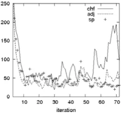
Fig. 5. Sample objective functions resulting from three filters CHF, ACHF(SP), ACHF(ADJ)

TABLE I

ERROR REDUCTION(IN PERCENTAGE)ACHIEVED BYACHF(SP)AND ACHF(ADJ)

ER1(%) ER2(%)

J 22,1 26,2

eu(p) 12,9 18,8

eu(f) 15,4 20,4

ev(p) 15,6 19,6

ev(p) 14,5 18,6

euv(p) 16,7 21,1

euv(f) 15 19,6

VII. NUMERICAL RESULTS

A. Adaptive CHF

In Table I the the error reductions by ACHF(ADJ) (using gradient measurements computed by adjoint equation) and by ACHF(SP) (SPSA using measurements of cost function) are displayed where ER1(%), ER2(%), expressed in percentage, show how the corresponding ACHF(SP) or ACHF(ADJ) has reduced rms (root-mean square) of estimation errors compared to that of CHF. For example, over the large windowk∈[5 : 72], the SPSA algorithm has reduced about 15%rms errors whereas this percentage is of order 20 % if the gradient is computed by the adjoint code. Figure 5 depicts instantaneous values of the objective function resulting from three filters.

To see in detail what happens really during the period of last four months, i.e. k ∈ [61 : 72], Table II dis-plays the RMS-PE and RMS-FE resulting from three filters. As expected, the ACHF(SP) behaves now better than the ACHF(ADJ), with the reduction of velocity error by more than 10 %. As to the CHF, during this period one observes an important increase of estimation error (see Fig. 5).

TABLE II

RMS OF ESTIMATION ERRORS AVERAGED OVERk∈[61 : 72]

Filter CHF ACHF(SP) ACHF(ADJ)

J(cm) 11.53 5.48 7.02

eu(p)(cm/s) 9.25 5.03 5.88

eu(f)(cm/s) 7.57 4.49 5.04

ev(p)(cm/s) 9.36 5.28 6.15

ev(f)(cm/s) 8.05 4.72 5.28

euv(p)(cm/s) 8.94 4.96 5.78

euv(f)(cm/s) 7.51 4.43 4.96

TABLE III

RMS OF ESTIMATION ERRORS AVERAGED OVERk∈[5 : 72]

Filter PEF APEF(SP) APEF(ADJ) ER1 (%) ER2 (%)

J 6.36 5.90 5.88 7.2 7.5

eu(p) 5.69 5.42 5.34 4.7 6.2

eu(f) 4.77 4.48 4.45 6.1 6.7

ev(p) 5.74 5.43 5.36 5.4 6.6

ev(f) 5.10 4.83 4.79 5.3 6.1

euv(p) 5.57 5.24 5.20 5.9 6.6

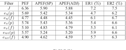
euv(f) 4.90 4.62 4.59 5.7 6.3 TABLE IV

RMS OF ESTIMATION ERRORS AVERAGED OVERk∈[61 : 72]

Filter PEF APEF(SP) APEF(ADJ) ER1(%) ER2(%)

J 6.94 5.75 5.96 17.1 14.1

eu(p) 5.99 5.04 5.23 15.9 12.7

eu(f) 5.26 4.44 4.59 15.6 12.7

ev(p) 6.19 5.19 5.41 16.2 12.6

ev(f) 5.47 4.56 4.82 18.5 11.9

euv(p) 5.85 4.92 5.11 15.9 12.6

euv(f) 5.15 4.32 4.52 16.1 12.2

[image:6.595.41.283.54.151.2]

B. Adaptive PEF

Table III-IV show that the PEF is much more efficient than the CHF and it slightly outperforms the ACHF(SP) and ACHF(ADJ). Thus the statistics extracted from DPE samples play the important role in correct estimating the filter gain and in improving the filter performance.

As the errors in the PEF are much lower than those produced by the CHF, there remains no great margin for reducing the errors in the PEF by adaptation compared to the case of optimizing the CHF structure. Even though, as seen in Tables III-IV, the adaptation remains still as advantageous tool for improving the performance of the PEF. For the assimilation period, compared with the PEF, the adaptation allows to reduce the rms estimation error by about 5-6%in the APEF(SP) and 6-7%in the APEF(ADJ). These reductions are less important than that achieved by the ACHF(SP) and ACHF(ADJ) with respect to the CHF (they are equal to 15 % and 20 % respectively, see Table I). At the last 4 months of assimilation, the APEF(SP) again outperforms the APEF(ADJ). Meantime, the error reduction is achieved by 16-17% in the APEF(SP) and by 12-13 % in the APEF(ADJ) compared to the non-adaptive PEF. The performance of the APEF presented here is based on the gain parametrization consisting of each parameter for each layer thickness. Due to space limit of this paper we cannot present here the way to parametrize the gain in 3d space. In this situation the number of parameters to be updated in the gain is equal to 140x180x4 = 100800 elements. By this way one can reduce more efficiently the filtered errors at the same computational cost as shown in this paper for 4 parameters since the SPSA uses simultaneous perturbations to approximate the gradient vector. We do hope to present these interesting results in an expanded version of this paper.

VIII. CONCLUSIONS

The objective of this paper is to present a very simple tool named as SPSA for optimization problems in very high dimensional systems and to demonstrate its high efficiency in state-parameter estimation problems which are typically

encountered in the field of data assimilation in meteorology and oceanography. The SPSA algorithm is very simple to implement since it requires only two integrations of direct numerical model for estimating the gradient of objective function. For meteorological and oceanic models with di-mension of order107−108, this method represents a great advantage for future development of optimal assimilation systems. As seen from the numerical experiments, due to a random simultaneous perturbation of all parameters, the SPSA requires more iterations, compared to the adjoint method, to well determine descent direction and to minimize the objective function. On the other hand, the SPSA method seems to be more efficient as iteration progresses, especially in optimizing non-linear systems since it calculates deriva-tives using the difference between two non-linear integrations of the model whereas the adjoint method approximates the gradient by linearization technique. That is why we found in all experiments the better performance of the AF based on SPSA at the end of assimilation period, compared to that based on the adjoint method.

REFERENCES

[1] M. Ghil and P. Manalotte-Rizzoli, ”Data assimilation in meteorology and oceanography”.Adv. Geophys, 33, pp. 141-266, 1991.

[2] A.E. Bryson and Y.C. Ho,Applied optimal control. Washington, DC: Hemisphere, 1975.

[3] H.S. Hoang, P. De Mey, O. Talagrand and R. Baraille, ”A new reduced-order adaptive filter for state estimation in high dimensional systems,” Automatica, 33, pp. 1475-1498, 1997.

[4] YA. Zypkin,Adaptation and Learning in Automatic Systems, New York, Academic, 1971.

[5] H.S. Hoang, O. Talagrand and R. Baraille, ”On the design of a stable filter for state estimation in high dimensional systems”,Automatica, 37, pp. 341-359, 2001.

[6] H.S. Hoang, O. Talagrand and R. Baraille, ”On the stability of a reduced-order filter based on dominant singular value decomposition of the systems dynamics”,Automatica, 45, pp. 2400-2405, 2009. [7] H.S. Hoang, O. Talagrand and R. Baraille, ”On an adaptive filter

for altimetric data data assimilation and its application to a primitive equation model MICOM”,Tellus, 57A, no 2, pp. 153-170, 2005. [8] C.S. Spall, ”An Overview of the Simultaneous Perturbation Method for

Efficient Optimization”,Johns Hopkins Apl Tech. Digest, V. 19, No 4, pp. 482-492, 1998.

[9] R. Todling and S.E. Cohn, ”Suboptimal schemes for atmospheric data assimilation based on the Kalman filter”,Mon. Wea. Rev., 122, pp. 2530-2557, 1994.

[10] G.H. Golub and C.F. Van Loan C.F., Matrix Computations, 2 edn. Johns Hopkins, 1993.

[11] T.M. Hamill, ”Ensemble-based atmospheric data assimilation”, in Predictability of Weather and Climate, Cambridge Univ. Press, 2006, pp. 124-156.

[12] G. Evensen G., ”The ensemble Kalman filter: Theoretical formulation and practical implementation”,Ocean Dynamics, 53, pp. 343-367, 2003. [13] R.E. Bellman and R.E. Kalaba, Quasi-linearization and non-linear

boundary-value problems, Elsevier, New-York, 1965.

[14] M. Cooper and K. Haines, ”Altimetric assimilation with water property conservation”,J. Geophys. Res., 101, pp. 1059-1077, 1996.