Keywords—Supply Chain Management (SCM), Logistics, Fixed Charge Transportation Problem (FCTP), Adaptive Genetic Algorithm, Fuzzy Logic Controller (FLC)
Abstract—Competitive global markets oblige the firms to reduce their overall costs while maintaining the same customer service level and this can be achieved just through a precise and efficient management of their supply chain network. The Fixed Charge Transportation Problem (FCTP) which is a more comprehensive type of Transportation Problem (TP) has several applications from different aspects in this network. Since the problem is NP-hard and solving this problem with decisive methods and heuristics will be computationally time consuming and expensive, two Genetic Algorithm are applied for this problem and also two fuzzy logic controllers are developed to automatically tune two critical parameters (Pc and Pm) of one of these two GAs.
Finally the results from the simple conventional GA and automatically tuned GA are compared together. This comparison demonstrated that the GA that is tuned with FLC reach the local optimum remarkably faster.
I. INTRODUCTION
N nowadays globalized markets, since the competitiveness is dreadfully increasing, supply chain design has been gaining importance and attention [2]. Companies have to at least keep the same customer service level, while the market’s competitiveness forces them to reduce their overall costs to maintain their profit margins.
A Supply Chain (SC) is a network of facilities and distribution centers that is responsible for procuring the materials, making intermediate and finished products out of those materials, and distributing the products to customers, and Supply Chain Management (SCM) is the strategy of integrating these functions together in order to facilitate the synchronization of all parts of this chain. A supply chain
Manuscript received December 8, 2010.
Zalinda Othman is with Industrial Computing Department, Faculty of Information Science and Technology, National University of Malaysia (UKM), 43600 Bangi, Selangor, Malaysia.
Mohammad-Reza Rostamian Delavar is now with Industrial Computing Department, Faculty of Information Science and Technology, National University of Malaysia (UKM), 43600 Bangi, Selangor, Malaysia (corresponding author to provide e-mail: mr.delavar@ gmail.com).
Sarah Behnam is with Production Engineering Department, School of Industrial Engineering and Management, KTH Royal Institute of Technology, Stockholm, Sweden.
Sina Lessanibahri is with Manufacturing and Industrial Engineering Department, Faculty of Mechanical Engineering, University Technologi Malaysia (UTM), 81310 Skudai, Johor Bahru, Malaysia.
network consists of five major chains: R&D chain, purchasing chain, production chain, quality chain and logistic chain [20, 21].
Indubitably logistic chain is an important function of business and is evolving into strategic supply chain management. Logistics is often defined as the art of bringing the right amount of the right product to the right place at the right time and usually refers to supply chain problems [13].
Among logistics activities, transportation network design provides a remarkable potential to reduce the overall costs and also to improve the service level. The transportation problem (TP) is a well-known basic network problem which was originally proposed by Hitchcock [1]. This problem is a very complicated supply chain problem and is considered as NP-Hard problem [20, 21].
In order to make the transportation problem more practical, many research papers assume that a fixed cost is also incurred along with variable cost of each commodity. The Fixed Charge Transportation Problem (FCTP) is introduced in the origins of the Operations Research [17]. In a FCTP, a single commodity is shipped from origin (source, supply) locations to destination (sink, demand) locations. The objective is to find the combination of routes that minimizes the total variable and fixed costs while satisfying the supply and demand requirements of each origin and destination. While similar to the transportation problem, the FCTP is much more difficult to solve due to the presence of fixed costs which causes discontinuities in the objective function [19]. It has been shown that this problem is an NP-hard problem [17]. Since the problem is NP-hard, the computational time to obtain exact solution increases in a polynomial manner and very quickly becomes extremely difficult and long as the size of the problem increases.
Some old researches have turned to heuristic algorithms for solving FCTP because the methods are constrained by limits on computer time. Adlakha and Kowalski [3] proposed a simple heuristic algorithm for solving a small FCTP, which was more time consuming than the algorithms for solving a regular transportation problem. Glover, Amini, and Kochenberger [18], developed a parametric ghost image processing for this problem. Many researches consider the problem as mixed integer programming and solve it with the solutions such as the branch-and-bound and the cutting plane methods, but these methods are generally inefficient and computationally expensive [4], as
Adaptive Genetic Algorithm for Fixed-Charge
Transportation Problem
Zalinda Othman, Mohammad-Reza Rostamian Delavar, Sarah Behnam, Sina Lessanibahri
they did not take advantage of special network structure of FCTP.
Different encoding schemes and representations are used for the Fixed-Charge Transportation Problems. Gottlieb, and Paulmann [16] developed and compared two GAs, one with permutation representation and another with matrix representation and at last they come to conclusion that GA with matrix representation yield better results. Gen, Li, and Ida [5], utilized the Prüfer number encoding to propose the spanning tree-based genetic algorithms for fixed-charge transportation problems. Su, and Zhan [15] developed a Genetic Algorithm with the sorted set of edge(S-ES) encoding scheme.
Jo, Li, and Gen [7] proposed a new feasibility criteria and repairing procedure for spanning-tree based chromosomes in GA. However Hajiaghaei-keshteli, Molla-Alizadeh-Zavardehi, and Tavakkoli-moghaddam [12], designed the chromosomes just with feasible solutions, which saved the computational time of repairing procedure in previous works. They also utilized the Taguchi experimental design to apply a robust calibration and ensure the best performance of the GA.
Since adjusting the crossover and mutation ratios has a great effect on GA’s performance, a Fuzzy Logic Controller is also applied to automatic fine tuning of these ratios, according to Wang, Wang, and Hu [8].
II. MATHEMATICAL MODEL
The FCTP can be considered as a distribution problem in which there are m sources (suppliers, warehouses or
factories) and n destinations (customers or demand points).
Shipping the commodities are possible from each of the m
sources to any of the n destinations at a shipping cost per
unit cij (unit cost for shipping from source i to destination j)
plus a fixed cost fij, adopted as route’s founding cost. Each
source i = 1, 2, . . . , m has ai units of supply, and each
customer j = 1, 2, . . . , n has a demand of bjunits. The
objective is to determine which routes are to be established and the size of the shipment on those routes, so that the total cost of satisfying the supply constraints, in order to meet the demands, is minimized. Standard FCTP formulation is shown as follows:
Minimize
∑∑
= = + = m i n j ij ij ij ijx f y
c Z 1 1 ), . . ( Subject to: n j b x j m i
ij 1,...,
1 = ≥
∑
= m i a x i n jij 1,...,
1 = ≤
∑
= 0 , ≥∀i j xij
0
0 =
= ij
ij if x
y
0
1 >
= ij
ij if x
y
where xij is the unknown variable to be shipped on the route
(i, j) from supplier i to customer j, cij is the shipping cost
per unit from supplier i to customer j. ai is the number of
units available at supplier i, and bj is the number of units
demanded at costumer j. The transportation cost for
shipping per unit from supplier i to customer j is cij×xij. fij is
the fixed cost related to route (i, j). The transportation
problem assumed to be balanced in this paper, as the unbalanced problems could simply be converted to balanced one, through adding a dummy supplier or a dummy customer.
III. GENETIC ALGORITHM
As the problem proved to be NP-hard [17], and due to taking too much time to consider all the possible combinations, utilizing the conventional methods can only be applied for the small size problems with a few number of variables. In this case, a genetic algorithm is developed for this problem.
The GA searches a problem space with a population of chromosomes, each of which represents an encoded solution. A fitness value is assigned to each chromosome according to its performance in which the more desirable the chromosome, the higher the fitness value becomes. The population evolves by a set of operators until some stopping criterion is met. A typical iteration of a GA, a generation, proceeds as follows. The best chromosomes of the current population are copied directly to the next generation (reproduction). A selection mechanism chooses chromosomes of the current population in such a way that the chromosome with the higher fitness value has a greater probability of being selected (roulette wheel). The selected chromosomes mate and generate new offspring (crossover). After the mating process, each offspring might mutate by another mechanism called mutation. The new population is then evaluated again, and the whole process is repeated [14].
A. Representation
The spanning-tree based representation is used for genetic chromosomes since it would be appropriate for transportation problems. Gen and Cheng [6], introduced the use of the Prüfer number which can equally and uniquely represent all the possible trees in a network graph, for solving various network problems.
In this paper, the Prüfer number is created from randomly generatedm+n−2digits in range [1, m+ n]. The Prüfer
number would be considered feasible only if the number of connected arcs to suppliers’ side is equal to the number of connected arcs to customers’ side, which is formulated as follows:
∑
∑
+ + = = + =+ m n
m i i m i i L L 1 1 ) 1 ( ) 1 (
it. They save the time by eliminating the need for recognizing the infeasible solutions and repairing them by generating only feasible chromosomes. They convert the above formula to the following formulas:
∑
=
− =
m
i i n
L
1 1
and
∑
++ =
− =
n m
m i
i m L
1 1
A string of n-1 digits from set of suppliers and a string of m-1 digits from set of customers are generated randomly,
and finally the two produced strings are combined together at random to design a feasible chromosome.
The uniqueness of the Prüfer number for a special shipment strategy can be determined through decoding it. The same decoding procedure as [12] is utilized in this paper:
Step 1: Let P(T) be the original Prüfer number and let P'(T) be the set of all the nodes that are not part of P(T) and designed as eligible for consideration.
Step 2: Repeat the following process – (2.1) – (2.5) – until no digits are left in P(T).
2.1 Let i be the lowest numbered eligible node in
P'(T). Let j be the leftmost digit of P(T).
2.2 If i and j are not in the same set O or D, add the
edge (i, j) to tree T. Otherwise, select the next
digit k from P(T) that is not included in the same set with i, exchange j with k, and add the edge
(i,k) to the tree T.
2.3 Remove j (or k) from P(T) and i from P'(T). If j
(or k) does not occur anywhere in the remaining
part of P(T), put it into P'(T).
2.4 Assign the available amount of units to xij = min{ai,bj} (or xik = min{ai, bk}) to the edge (i,j)
or (i,k)) where i
∈
O and j, k∈
D.2.5 Update availability ai =ai–xij and bj = bj–xij (or
bk = bk–xik).
Step 3: If no digits remain in P(T) then there are exactly two nodes, i and j, still eligible in P'(T) for
consideration. Add edge (i, j) to tree T and form a
tree with m+n−2edges.
Step 4: If there are no available units to assign, then stop. Otherwise, there are y plants with a>0 units, and z
costumers with b>0 demands yet. One of these states occurs:
I. If y=1and
z
=
1
, Add the edge betweenthe plant and the customer to the tree and assign the available amount to the edge. II. If y>1 and
z
=
1
, Add the edge betweenthe plants and the customer to the tree and assign the available amount to the edge.
III. If y=1 and
z
>
1
, Add the edge betweenthe plant and the customers to the tree and assign the available amount to the edge. IV. If y>1 and
z
>
1
, Consider them as anew transportation model with y plants
and z customers, then generate Prüfer
number, and Repeat step 1 to 4.
If a cycle exists; remove the edge that is assigned zero flow. A new spanning tree is formed with m+n−2edges.
B. Initialization
Each generated chromosome is considered as an individual solution to the problem. In the first generation chromosomes are generated as many as population size. The random method is applied for generating the initial population.
C. Selection mechanism
As the total transportation cost including variable and fixed costs should be minimized in this problem, better solutions are those results with lower objective functions. The higher fitness value considered the better chromosome, so the applied function is formulated as follows:
Function Objective
1 Value
Fitness =
Since the Roulette-Wheel selection mechanism is deployed, the chromosomes with higher fitness values have more chance to be selected.
D. Genetic operators Reproduction
The pr% of the chromosomes with higher fitness values are transferred to the next generation (elite strategy).
Crossover
Crossover combines the two selected chromosomes’ features in order to create two better offsprings. The remaining (pc=1-pr%) of the chromosomes in next generation going to be generated from crossover operation. The one-point crossover is used in the algorithm in such a way that the feasibility criterion has been met. It means that after selecting the point from which the parents are separated into two different parts, the first parts are directly copied to the associated offspring, but the second part is inherited from the opposite parent, regarding the two previously mentioned feasibility criteria.
Mutation
The mutation operator is an important process of any successful GA that reorganizes the structure of the genes so that the algorithm can escape from searching just in local optimum area. It can also be regarded as a simple local search technique.
mutation operation is going to be performed. The inversion mutation is utilized in this paper. In this operator two genes are randomly selected from an offspring and their positions are inverted. Since the chromosomes are feasible after crossover, the mutated offsprings are also going to be feasible.
IV. FUZZY LOGIC CONTROLLER
Being one of the most popular applications of Lotfi Zadeh’s Fuzzy Set Theory [11], Fuzzy Logic Controllers (FLCs) are demonstrated initially by Mamdani [10] in 1974. FLCs are knowledge-based controllers that are usually derived from a knowledge acquisition process or are automatically synthesized from a self-organizing control architecture [9].
Creating a balance between exploration and exploitation plays a significant role in GA’s performance. Therefore, regulating the GA parameters such as population size, number of generations, crossover probability, and mutation probability is one of the crucial subjects for providing this balance.
Two FLCs are used for automatically tuning the pc and
pm based on the changes in the average fitness of the population [8]. Let ∆f(t) be the difference between average fitness function of the tth and t-1th generations and ∆f(t− 1) be the difference between t-1th and t-2th generations, then the crossover and mutation ratios for the next generation is done using the following IF–THEN concept:
• If |∆f(t)− ∆f(t−1)| <ε, is a small positive number near to zero), then rapidly increase the pc and pm for the next generation.
• If ∆f(t)− ∆f(t−1) <−ε then decrease the pc and pm for the next generation.
• If ∆f(t)− ∆f(t−1) >ε then pc and pm for the next generation.
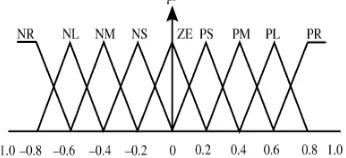
[image:4.612.348.533.53.256.2]The inputs for both FLCs are ∆f(t) and ∆f(t−1). The output for one FLC is the change in crossover ratio, ∆c(t), and for another one is the change in mutation ratio, ∆m(t). The membership functions of two inputs are illustrated in fig. 1, the membership function of ∆c(t) is illustrated in fig. 2, and the membership function of ∆m(t) is illustrated in fig. 3.
After obtaining the inputs, ∆f(t) and ∆f(t−1), from GA, the FLC sets the inputs to their associated membership functions. According to available rules in fuzzy decision table, which is shown in table.1, a fuzzy value is extracted from each of the nine membership functions, and at last these function values are converted to one crisp output for each FLC.
Table 1 Fuzzy Decision Table
∆f(t−1)
NR NL NM NS ZE PS PM PL PR
∆f(t)
NR NR NL NL NM NM NS NS ZE ZE
NL NL NL NM NM NS NS ZE ZE PS
NM NL NM NM NS NS ZE ZE PS PS
NS NM NM NS NS ZE ZE PS PS PM
ZE NM NS NS ZE PM PS PS PM PM
PS NS NS ZE ZE PS PS PM PM PL
PM NS ZE ZE PS PS PM PM PL PL
PL ZE ZE PS PS PM PM PL PL PR
PR ZE PS PS PM PM PL PL PR PR
After achieving the outputs, the crossover probability and mutation probability for the next generation, t+1, is
calculated through following equations:
𝑃𝑃𝑃𝑃(𝑡𝑡+ 1) =𝑃𝑃𝑃𝑃(𝑡𝑡) +∆𝑃𝑃(𝑡𝑡)
𝑃𝑃𝑃𝑃(𝑡𝑡+ 1) =𝑃𝑃𝑃𝑃(𝑡𝑡) +∆𝑃𝑃(𝑡𝑡)
where Pc(t) is the crossover ratio at generation t, and Pm(t)
is the mutation ratio at generation t.
Fig. 1. The membership function for both inputs: ∆f(t−1)
and ∆f(t)
Fig. 2. The membership function for the output ∆c(t)
Fig. 3. The membership function for the output ∆m(t)
[image:4.612.82.255.578.657.2]V. NUMERICAL EXPERIMENTS
In order to investigate the proposed algorithm’s effectiveness and efficiency, its results are compared with the results obtained from simple GA (without FLC).
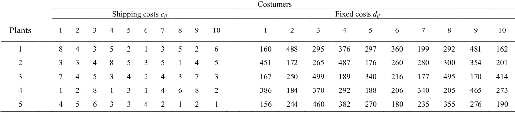
[image:5.612.328.556.184.349.2]The problem sizes, stopping criterion, and population size are the same as Jo, Li, and Gen [7]. The problem sizes, total supplies (or total demands) and the ranges of the fixed costs which are generated randomly are demonstrated in table 2. The unit variable costs are integer values in the range 1 to 8 in both test problems which are shown in tables 3 and 4.
Table 2. Total supply (demand) and ranges of fixed cost Problem size
(m×n) Total supply Range of fixed cost
4×5 275 [50,100]
5×10 1485 [150,500]
Each problem size is run 10 times. Other genetic algorithm parameters that are common in both test problems are, population-size= 100, Pc= 0.5, and Pm= 0.3. The maximum number of generation in this test problem is 500.
The local optimal solution with the objective function of 1484 was found in both algorithms, but with a major difference. Running each algorithm ten times, the average generation number for getting to this local optima was 43 for the GA-FLC, while it was 72 for the simple GA. This is illustrated in fig. 4.
For the test problem 2, which has the size 5×10, the maximum number of generations is 1000.
Running both algorithms for test problem 2, the comparative result is represented in fig. 5. As it can be perceived from this figure, GA-FLC has more expeditious steps towards the local optima. Additionally, the simple GA represents 6442 as the average of best objective functions after running for 1000 generations; while the GA-FLC performs better and exhibits 6406 as its final outcome.
VI. CONCLUSION AND FUTURE WORKS
This paper considered a transportation network between two parties in a supply chain, i.e supplier and customer, and
tried to reduce the overall transportation costs to its minimum point, regarding both variable (per shipping product) and fixed (per route) costs, in such a way that all supply constraints, and also all demand constraints should be satisfied.
The spanning-tree based genetic algorithm was employed to solve the non-linear fixed charge transportation problem, which is considered to be NP-hard and couldn’t be solved by traditional methods. For obtaining better results from GA, a Fuzzy Logic Controller is also employed to automatically tune the crossover probability and mutation probability of the algorithm. Comparing the simple GA and the GA with FLC, the latter showed an outstanding speed towards finding the local optimum.
Since FCTP is a kind of network model that can be used in several various fields such as transportation, computer science, manufacturing, decision support systems, scheduling, and etc., there are great potential opportunities
for developing further research in this field, for instance tuning more critical parameters from a genetic algorithm dynamically, such as population size or maximum number of generations, or creating a heuristic to find an appropriate initial population, or even adding a local search technique like simulated annealing to genetic algorithm.
1480 1490 1500 1510 1520
0 100 200 300 400 500 GA-FLC GA
6400 6600 6800 7000 7200 7400
[image:5.612.41.295.210.246.2]0 200 400 600 800 1000 GA-FLC GA
Table 3. Unit variable cost and fixed costs in 4×5 problem Costumers
Shipping costs cij Fixed costs dij
Plants 1 2 3 4 5 1 2 3 4 5
1 8 4 3 5 8 60 88 95 76 97
2 3 6 4 8 5 51 72 65 87 76
3 8 4 5 3 4 67 89 99 89 100
[image:5.612.41.267.337.457.2]4 4 6 8 3 3 86 84 70 92 88
Fig. 4. Comparing GA-FLC and GA in test problem 1
[image:5.612.53.276.551.693.2]REFERENCES
[1] F.L. Hitchcock, “The distribution of a product from several sources to numerous localities”, Journal of Mathematical Physic 20, 1941, pp.224–230.
[2] D.J. Thomas, P.M. Griffin, “Coordinated supply chain management”, European Journal of Operational Research 94, 1996 pp.1–15, doi: 10.1016/0377- 2217(96)00098-7.
[3] V. Adlakha, K. Kowalski, “A simple heuristic for solving small fixed-charge transportation problems”, OMEGA: The International Journal of Management Science, 31, 2003, pp.205–211.
[4] D.I. Steinberg, “The fixed charge problem”, Naval Research Logistics Quarterly, 17, 1970, pp.217–236.
[5] M. Gen, Y. Li, and K. Ida, “Spanning tree-based genetic algorithm for bicriteria fixed charge transportation problem”, Journal of Japan Society for Fuzzy Theory and Systems, 12(2), 2000, pp.295–303. [6] M. Gen, and R. Cheng, “Genetic algorithms and engineering design”
NY: John Wiley and Sons, 1997.
[7] J. Jo, Y. Li, and M. Gen, “Nonlinear fixed charge transportation problem by spanning tree-based genetic algorithm”, Computers & Industrial Engineering, 53, 2007, pp.290–298.
[8] P.T. Wang, G.S. Wang, and Z.G. Hu, “Speeding up the search process of genetic algorithm by fuzzy logic”, Proceedings of the fifth European congress on intelligent techniques and soft computing, 1997, pp. 665–671.
[9] P.P. Bonissone, “Fuzzy logic controllers: an industrial reality”, computational intelligence: Imitating Life. J.M. Zurada, R.J. Marks II, C.J. Robinson (Eds.), IEEE Press, 1994, pp.316-327.
[10] E.H. Mamdani, “Application of Fuzzy Algorithms for Control of Simple Dynamic Plants”, Proceedings of IEE, Vol. 121, No. 12, 1974.
[11] Zadeh, L. A., “Fuzzy Sets, Information and Control”, Vol. 8. 1965. [12] M. Hajiaghaei-Keshteli, S. Molla-Alizadeh-Zavardehi, and R.
Tavakkoli-Moghaddam, “Addressing a nonlinear fixed-charge transportation problem using a spanning tree-based genetic algorithm”, Computers and industrial engineering, 59, 2010, pp.259– 271.
[13] B. Tilanus, “Introduction to information system in logistics and transportation”, Information System in Logistics and Transportation, ed. B. Tilanus, p s. city: Pergamon, Elsevier Science, Ltd, 1997. [14] D.E. Goldberg, “Genetic algorithms in search, optimization and
machine learning”, Reading, MA: Addison-Wesley, 1989.
[15] S. Su, D.C. Zhan,”New Genetic Algorithm for the Fixed Charge Transportation Problem”, Proceedings of the 6th World Congress on
Intelligent Control and Automation, 2006, pp.7039-7043.
[16] J. Gottlieb, and L. Paulmann, “Genetic algorithms for the fixed charge transportation problem”, Proceedings of IEEE international conference on evolutionary computation, Anchorage, 1998, pp.330– 335.
[17] W.M. Hirsch, and G.B. Dantzig, “The fixed charge problem”, Naval Research Logistics Quarterly, 15, 1968, pp.413–424.
[18] F. Glover, M. Amini,and G. Kochenberger, “Parametric ghost image processes for fixed charge problems: a study of transportation networks”, Journal of Heuristics, 11, 2005, pp.307–316.
[19] F. Glover, D. Klingman, and N.V. Phillips, “Network models in optimization and their applications in practice”, New York: Wiley, 1992.
[20] K.M. Chao, P. Norman, R. Anane, and A. James, “A chain based approach for engineering design”, Journal of Computers in Industry 48 (1), 2002, pp. 17–28.
[21] C. Savaskan, R.S. Bhattacharya, and L.N. Van Wassenhove, “Closed-loop supply chain models with product remanufacturing”,
[image:6.612.40.562.65.187.2]Management Science, Linthicum 50 (2), 2004, p. 239.
Table 4. Unit variable cost and fixed costs in 5×10 problem
Costumers
Shipping costs cij Fixed costs dij
Plants 1 2 3 4 5 6 7 8 9 10 1 2 3 4 5 6 7 8 9 10
1 8 4 3 5 2 1 3 5 2 6 160 488 295 376 297 360 199 292 481 162
2 3 3 4 8 5 3 5 1 4 5 451 172 265 487 176 260 280 300 354 201
3 7 4 5 3 4 2 4 3 7 3 167 250 499 189 340 216 177 495 170 414
4 1 2 8 1 3 1 4 6 8 2 386 184 370 292 188 206 340 205 465 273