Dynamical Characteristics of a Lateral Guided Robotic Vehicle with a Rear Wheel Steering Mechanism Controlled by SSM

Dynamical Characteristics of a Lateral Guided Robotic Vehicle with a

Rear Wheel Steering Mechanism Controlled by SSM

Yoshihiro Takita , Hisashi Date and Shinya Ohkawa

Abstract - This paper discuses sensor steering mechanism (SSM) for a laterally guided vehicle with a rear wheel steering mechanism. The authors have demonstrated the geometry of SSMs for front wheel steering type and reverse phase four-wheel steering type vehicles. SSMs allow stable lateral guiding performance for automated vehicles following a path with straight and curved portions created by a guideway. On other hand, no SSM has been established for a rear wheel steering type vehicle. Rear wheel steering vehicles include forklifts and backward moving conventional motor vehicles which are front wheel vehicles. A SSM for rear wheel steering vehicles would enable a forklift to move into any spaces using automation. This paper proposes a SSM relation for a rear wheel steering vehicle and describes the construction of experimental robotic vehicle with the proposed SSM. Simulated and an experimental data show the advantages of the proposed SSM.

Index Terms - Lateral Guide, Mobile Robot, Steering Vehicle, Rear Steer, Dynamical System, Drifting

I. INTRODUCTION

AGVs (automated guided vehicle) are used not only in factories but also in many other applications as a productive efficient labor and cost-saving device. The difficulty in using these vehicles to maintain their stability in the lateral direction when moving. This problem is the result of the dynamic characteristics of the sensor position and controlling mechanism. The practical speed limit of an AGV [1-4] used in manufacturing facilities is approximately 2 m/s. On the other hand, a dual mode truck (DMT) [5], which has been researched in recent years, is driven by a human operator on ordinary roads and is controlled automatically on roads that have been installed with mechanical guidance devices. However, the speed limit for stable tracking depends on the geometry of the guiding mechanism. From 2005 to 2007, the defense advanced research projects agency (DARPA) [6] held the DARPA Grand Challenges which spurred many robotics researchers to develop the first autonomous vehicle. The average speed of the top vehicle was approximately 30 km/h, which is still far short of that obtainable using a human driver. This competition has brought to light many technical problems to creating an autonomous vehicle. In the case of following the

Yoshihiro Takita, Dept. of Computer Science, National Defense Academy, Japan (e-mail: takita@nda.ac.jp)

Hisashi Date, Dept. of Computer Science, National Defense Academy, Japan (e-mail: date@nda.ac.jp)

Shinya Ohkawa, Graduate student, Dept. of Computer Science, National Defense Academy, Japan (e-mail: em50045@nda.ac.jp)

center line of the road, the important point is to control the steering angle without losing lateral stability.

The authors have proposed a sensor steering mechanism (SSM) for laterally guided vehicles with either front wheel [7] or four-wheel steering mechanisms [8]. When the vehicle is guided by the SSM, it has been shown that no speed limit exists for straight-line travel, except with respect to the oversteer characteristics. In addition, the experimental results obtained using a newly developed robotic vehicle revealed that the SSM can follow a guideway while adjusting the centrifugal force and the side force of the tires when turning. Furthermore, the previous paper derived the dynamic equations of motion and calculated the movement of the vehicle controlled by the SSM along with the experimentally measured tire characteristics. For the accurate simulation of a vehicle moving at high speed, the authors proposed a variable kinetic friction model of the tire and applied it to the derived dynamic equations [9]. The existence of the sensor arm prevents the application of the SSM to vehicles operating on ordinary roads. In the previous paper, this problem was solved by replacing the sensor arm with a miniaturized 1 kHz intelligent camera [10,11].

The current paper focuses on forklifts, which are widely used for cargo handling operations, however the SSM is not applied to this type of vehicle, which has its steering mechanism located at the rear. On the other hand, when a car backs up, it can be considered a rear wheel steering vehicle. If a SSM can be applied, an increase in speed laterally guided vehicles with rear steering mechanisms can be expected.

This paper proposed a SSM for rear wheel steering vehicles, and the ratio of steering angle and sensor arm angle is determined. An experimental vehicle is developed and tested on a test course. A dynamic model of the experimental vehicle is derived and applied to a variable kinetic friction tire model to simulate a trajectory of movement. Experimental results of high-speed movement and the moving simulation are presented. These results demonstrate that a SSM for rear wheel steering vehicles can perform at high speeds and maintain stability on a test course.

II. SSM AND THE DYNAMIC MODEL

A. SSM (Sensor Steering Mechanism)

A front wheel steering type SSM and the proposed rear wheel steering type SSM are shown in Fig. 1. It is assumed that backward movement of a front wheel steering vehicle is equivalent to a rear wheel steering vehicle. The front wheel steering type SSM and rear wheel steering type SSM consist of elements PQS_f and QPS_r, respectively. When the rear wheel steering type vehicle moves counterclockwise by the steering angle δ with steering radius R, then the front tire P moves on a radius Rbut the rear tire Qmoves off the test course. Here, S_f is the sensor on the front wheel steering type SSM, which follows the guideway exactly. Then the angle of sensor arm QS_f is 2δ. The triangles PQO and PEO are congruent to each other, and it is assumed that S_ris the point at which the circular arc intersects with segment EO. The relation between the sensor arm angle φ and steering angle δ is as follows:

δ = 2φ _{. (1)}

The sensor arm length PSr is PS_r = 2R sin δ

2 (2)

which is linearized around the equilibrium point as follows:

PSr≈ Rδ ≈L . (3)

As a result, the steering angle δ with the rear wheel steering type SSM is given by minus two times the sensor arm angle

φ.

B. Dynamic Equation of Motion

Figure 2 shows the rigid body bicycle vehicle model moving at velocity V. It is assumed that the right and left tires have the same characteristics. In Fig. 2, N is the Newton reference frame. Dextral sets of mutually perpendicular unit vectors n₁ and n₂ are fixed in N. The reference frame A is fixed on the vehicle, and the mutually perpendicular unit vectors a₁ and a₂ are constant relative to A. Here, θis the body position angle, g is the yaw angle, δ_f and δ_r are the steering angles of the front and rear tires, respectively, βfand β_rare the slip angles of the front and rear tires, respectively, and γ_f and γ_r are the angles between n₁ and the velocity vector of the front and rear axles, respectively. In addition, U_fand U_rare the cornering forces of the front and rear tires, respectively, l_fand l_rare the distances from the center of gravity to the front and rear axles, respectively, m is the mass, and I is the moment of inertia about the yaw-axis of the vehicle. Finally, F_f and F_rare the driving forces, and D_f and D_r are the rolling resistance forces of the front and rear tires, respectively. The dynamic equations of motion are as follows:

mx = - Ff cos (θ +δf ) - Uf sin (θ +δf )

- Ur sin (θ +δr) - Frcos (θ +δr)

- Dr (lr θ sinθ + Dr x)/E, (4)

my = Ff sin (θ +δf ) + Uf cos (θ +δf )

+ Ur cos (θ +δr ) + Fr sin (θ +δr )

+ D_r (l_r θ cos θ - y)/E_{, (5)}

Iθ = lf (Ff sin δf + Uf cosδf )

- lr (Frsin δr + Ur cosδr)

- lrDr(lr θ + xsin θ - ycos θ )/E . (6) Here,

E = x2+y2+l_r 2_θ2_+2l

r xθsin θ - 2lr yθcos θ.

In this case, the cornering forces are regarded as a linear function of the slip angle written as follows:

R δ δ

δ

δ

L

L

rear tire

front tire

(wheel base)

sensor or guideway

P Q

O S

E

L

δ

φ

sensor or guideway

S_r

f

Fig. 1 Schematic representation of SSM

n2

n1

N

lr

lf

δf βf

γ θ V

βr

2Uf

2Ur

dy dt

lf dθ_dt

dθ dt

-lr

A*_(x,y)  

γr

γf

δr a2 A a1

dx dt n1 dy

dtn2

a2 dx

dt n1

n2

a2 Y

X

Vf Ff

D_f

Vr

D_r

F_r

Fig. 2 Schematic diagram of a vehicle model

Uf = - 2Kfβf , Ur = - 2Kr βr (7) where K_f and K_rare the cornering power of the front and rear tires, respectively.

III SIMULATION OF RUNNING ON THE COURSE

A. Tire Characteristics

In the previous paper of the authors, the relationship between the lateral force and the slip angle was measured using test equipment. The next equations show the measured lateral forces generated by the tire when the contact forces are set to 3.63 N and 4.12 N. These data are approximated by fourth order polynomials by using the least squares method:

U₁ static(β) = -2.146 × 10-5_β4 _{+ 1.824 × 10}-3_β3

-5.923 × 10-2_β2 _{+ 0.958 β + 8.391 × 10}-2

(8)

U₂ static(β) = -2.542 × 10-5_β4 _{+ 2.183 × 10}-3_β3

-7.066 × 10-2_β2 _{+ 1.118 β + 5.146 × 10}-2

. (9) Equation (8) is equivalent to equation (9) multiplied by the contact force ratio 4.12/3.63. In this case the cornering force is proportionate to the contact force of the tires. For the simulation, twice the cornering force is applied to the body because the front and rear axles have two wheels each. B. Variable Kinetic Friction Model of Tires

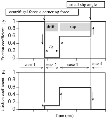
proposed for simulating the drifting cornering motion at high speed. Case 1 invokes static friction only, not slipping between the tires and the ground, and the cornering forces U_f and U_r are approximately equal to the values given by equations (8) and (9). Case 2 is drifting, which involves slipping between the tires and the ground. Although Case 2 involves two sets of forces, i.e., the friction force acting in the direction opposite to the velocity vector of the tires and the cornering force, which is small because the direction of movement of the vehicle is not affected by the steering angle. These sets of forces use friction coefficient µ_k and friction coefficient µ_f, respectively. For drifting (Case 2), the cornering force must be smaller than the centrifugal force of the body at high speed. The drifting time is

T_d. Case 3 is slipping, which involves sliding between the tires

and the ground. The types of friction forces involved are identical to those of Case 2, but not the magnitude of the forces. This case starts T_dafter the beginning of Case 2. Case 4 is identical to Case 1. When the slip angle becomes small, the vehicle stops slipping (Case 3) and only static friction is involved (Case 4). When the front and rear wheels slide at the same time, control of the vehicle orientation becomes impossible. It is therefore assumed that only the rear tires drift (Case 2). The friction force D_r and cornering force U_rof the rear tires are as follows:

Dr = Wrμk (10)

Ur= 2μf Ur static(βr) (11) where W_r and U_rstatic are the contact force and the cornering force.

C. Simulation Conditions

The test course, which consists of two semicircles of radius 0.5 m connected by straight segments of length 0.7 m, was used to analyze the turning motion, including drifting, of a vehicle laterally guided by the SSM. Dynamic analysis of the vehicle was performed by integrating equations (4) to (6) with the Runge-Kutta method. The calculation results for the center of gravity of the vehicle and the contact points of the guideway and the sensor were determined using the SSM. In addition, the calculated velocity vectors and the steering angles of the front and rear tires were used to determine the slip angles and cornering forces.

For the simulation, physical parameters of rear wheel steering type robotic vehicles are shown in Table 1. H is the height of the center of gravity above the road surface, b is the tread width, W_f and W_r are the loads on the front and rear tires, respectively. In addition, the initialization parameters of the numerical values are shown in Table 2. The driving force can be obtained using the equation of motion by setting F_f= 0 for the vehicle. The supplied current to the DC motor is set to a constant value, and the driving torque of the driven wheel is defined by the angular velocity and torque relations of the DC motor as follows:

Fdrive= (Nf - 60Vdrivend 2πr)

Nf T_m

n_d

r_{tire (12)}

where F_driveis the driving force, N_fis the no-load speed of the motor, V_driveis the speed of the driving wheel, n_dis the gear ratio, r_tireis the tire radius, and T_mis the stalling torque of the motor. Table 3 shows the parameters of the DC motor used for the simulation. Here, the tire radius r_tireand the gear ratio

n_dare 0.0295 m and 4.57, respectively.

small slip angle

centrifugal force > cornering force

0 0.2 0.4 0.6 0.8 1 0 0.2 0.4 0.6 0.8 1

Friction coefficient

μf

Time (sec)

Friction coefficient

μk

case 2

Td

case 1

slip drift

case 4 case 3

Fig. 3 Prediction of friction model

The cornering forces of this vehicles are

Uf = 2U1 static(βf)μs (13)

Ur = 2U2 static(βr)μf . (14)

Here, µ_s is used to compensate the measured tire characteristic and the friction coefficient of the road surface. An arbitrary value is used in the simulation. In addition, the compensation parameter of rear tires is included in µ_f.

D. Simulation Results

The simulation is started from an initial point at speed 2.0 m/s as shown in Table 2. The calculated trajectory is made close to the experimental result by changing friction parameters µ_s and µ_f. Note, no simulation was made below a speed of approximately 1.3 m/s, because the drift condition does not appear at low speed. Figure 4 shows the simulated results of the rear wheel steering type of SSM with friction parameters shown in Table 1. In this figure, (a), (b), (c) and (d) show the trajectories, velocities of front and rear axles, steering angle, front tire slip angle and rear tire slip angle, respectively. This figure shows that a large steering angle is made at each entrance of a curve and a drift is briefly generated (as indicated by a large slip angle), and the moving speeds of the front and rear axles decrease while the rear axle is outside the test course. The trajectory of the front axle stays on the test course and the vehicle achieves a stable running state. Thus, accurate simulation results give information on effective characteristics of a controlled vehicle.

IV. EXPERIMENTAL SETUP AND RESULT S

-0.6 -0.4 -0.2 0 0.2 0.4 0.6

-1.25 -1 -0.75 -0.5 -0.25 0 0.25 0.5

Y (m)

X (m)

rear

front guideway

(a) trajectory

1.8 2 2.2 2.4 2.6

0 0.5 1 1.5 2 2.5 3 3.5

Velocity (m/s)

Time (sec)

rear

front

(b) speed

-35 -30 -25 -20 -15 -10 -5 0 5 10

0 0.5 1 1.5 2 2.5 3 3.5

Steering angle (deg)

Time (sec)

(c) steering angle

-25 -20 -15 -10 -5 0 5

0 0.5 1 1.5 2 2.5 3 3.5

Slip angle (deg)

Time (sec)

rear front

(d) slip angle

Fig. 4 Simulated result of running on the test course

lateral control of the rear wheel steering type vehicle is achieved by the SSM method. The physical parameters of this vehicle are the same as in the simulation.

The rotational angle of the CMOS camera is controlled by a servo motor through the deceleration gear. The rear steering angle is controlled by a radio control servo motor in which the original control circuit has been replaced by a specially built controller. In order to achieve perfect Ackerman steering geometry, a small improvement to the original vehicle body (made by Tamiya Inc.) was necessary. The body is a monocoque structure made of plastic. A double wishbone suspension is adapted to the body, but the effect of suspension is not included in the dynamic simulation. The vehicle is equipped with tread-patterned soft rubber tires, the insides of

Table 1 Parameters of vehicle

I 5.8 ×10-3 _{kg m}2 l_f 0.075 m

m 1.378 kg l_r 0.15 m

L 0.225 m b 0.134 m

H 0.050 m W_r 4.49 N

W_{f 9.02 N}

Table 2 Initial values for simulation

V 2.0 m/s

A (x, y) ( - 0.5 m, - 0.5 m )

θ 0.0 rad

Table 3 Estimated friction parameter

case 1 μs 0.9 μf 1 μk 0

T_d

-case 2 drift slip 0.72 0.72 0.01 0.54 0.01 0.81 0.018 sec

-Fig. 5 Experimental view of developed SSM robot vehicle

L = 0.225

battery

1kHz Smart Camera

Observed point

L = 0.225

Lamp

control system

differential gear

motor 1

motor 2 motor 3

φ 2φ

motor 1 motor 2

motor 3

Fig. 6 Construction of a rear wheel steering vehicle

with rotary encoder

H8S/2258F for driving SRAM EEPROM

serial interface

for camera

motor 1

motor 2

I/O port

down/up loading

Counter PWM TPU H8S/300H

CPU

core Odometer

1 kHz CMOS camera with potentiometer

for steering

motor 3

A/D

Fig. 7 Control system for rear wheel steering SSM

B. Control System

The construction of this controller is shown in Fig. 7. The robot control system is constructed with a H8S/2258F one-chip microcomputer (Renesas Technology) and is installed at the rear of the vehicle. The 1 kHz intelligent camera captures one 8-bit image with 128×128 pixels per millisecond. The sensor chip has 8 bit AD converters and charge amplifiers for each row column, and can convert all 128 pixels in one line simultaneously. One image frame can be processed by repeating this operation 128 times. The size of this CMOS image sensor is 7.4×11.2 mm. A 1 kHz frame rate is achieved using a field programmable gate array (FPGA). Verilog HDL is used as the programming language of the FPGA, which is programmed so that the microprocessor can access image data. C. Experimental Conditions

For the experiment, a test course was built having a 0.02 m wide strip of white tape on a black road surface. The geometry of the test course was identical to that used in the simulation. The surface material was constructed using acrylic film. Comparison of the simulated and experimental results required the measurement of the locus of the actual robot. Experimental data were acquired using a ProReflex (Qualisys) three-dimensional motion capture system having a sampling rate of 240 per second and a measuring error within ±0.2s mm. This measurement system captures the three-dimensional position of two reflecting markers attached to centers of the front and rear axles, and the captured data is output to a text file. A constant pulse interval is applied to a motor-driving circuit to produce a constant force equivalent to in the simulation. In this experiment, the maximum speed of the vehicle was set to 2.2 m/sec, and the control program stores the steering angle and the control variables in the built-in RAM every 10 ms. After each experimental run, the data is uploaded to a personal computer.

D. Experimental Results

Figures 8 and 9 show results from experimental runs on the test course when the vehicle is moving at low speed and high speed. In these figures, (a) is the trajectories of front and rear axles, (b) is the speed of the front and rear axles, and (c) and (d) are the steering angle and the difference between the target value and the measured value uploaded by the robot controller, respectively.

At the low speed the front axle passes over the guideway and the rear axle moves outside the guideway loop in the manner shown in Fig. 1. Figure 8(b) shows that the speed of the rear axle is faster than that of the front axle because the rear axle is the outside the loop at the curve. Apparenlty, the front

part of the robotic vehicle moves at an approximately consant speed, experimentally confirming the effectiveness of the SSM control.

The more interesting results are obtained from the high-speed motion experiment. In Fig. 9(a), a tracking error appears the front axle and passes outside the guideway loop at the same time the rear axle is far outside the guideway loop. Neverthless, the robotic vehicle maintaines a stable running state on the test course. By comparing Figs. 4 and 9, one sees that the simulation result corresponds well with the high-speed motion experiment. The drift at the entrance of the curve was necessary to match the tracking error of the experimental results. According to the simulated results, the rear tires are steered sharply at the beginning of the curve, then the rear tires slip for a short time and move far from the guideway before the contact force is recovered. Figures 8(d) and 9(d) show the errors of the steering angle and target value given by the camera angle. Comparing Figs. 8(d) and 9(d), it is clear that a major cause for the error is a delay in the control system. Despite this problem, the SSM achieved a stable running state running on the test course at high speed.

V. CONCLUSIONS

This paper proposed a SSM to a laterally guide a rear wheel steering vehicle. The main idea of the SSM is that the sensor is located at the tip of a sensor arm that has the same length as the wheel base of the vehicle, and the steering angle is two times the sensor arm angle, but in the opposite direction. This relation is achieved by linear approximation. In this paper, a SSM robotic vehicle is developed and a dynamic model of a rear wheel steering vehicle is derived and calculated. The experimental and simulated results show that the proposed SSM achieves stable tracking even if the vehicle drifts at the beginning of curves. Furthers, experimental and simulated results correspond well with each other. Finally, the advantages of the proposed SSM are that the system is simple and stable behavior is achieved. Therefore, SSMs can be used not only in front wheel steering vehicles and reverse phase four-wheel steering vehicles but also in rear wheel steering vehicles.

REFERENCE

[1] Abe, M., Vehicle Dynamics and Control, [1979), pp.192-213. kyoritsu Publication(in Japanese)

[2] Minami, M., et al., Magnetic Autonomous Guidance b y Intelligent Compensation System, Vol.31, No.5(1987), pp.382-391.

[3] Makino, T., et al., High-Speed Driving Control of an Automatic Guided Vehicle Using an Image Sensor, Trans of the SICE , Vol.28, No.5(1992), pp.595-603.

[4] Shladover, S.E., et al., Steering Controller Design For Automated Guideway Transit Vehicles, Trans of the ASME, Vol. 100, (1978), 1-8

[5] Tsunashima, H., A Simulation Study on Performance of Lateral Guidance System for Dual Mode Truck, Trans of the JSME, Series C, Vol.65, No.634(1999), pp.2279-2286. [6] http://www.grandchallenge.org/

-0.6 -0.4 -0.2 0 0.2 0.4 0.6

-1.25 -1 -0.75 -0.5 -0.25 0 0.25 0.5

Y (m)

X (m)

rear

front guideway

(a) trajectory

1.2 1.4 1.6

0 0.5 1 1.5 2 2.5 3 3.5 4 4.5 5 5.5

Velocity (m/s)

Time (sec)

rear

front

(b) speed

-35 -30 -25 -20 -15 -10 -5 0 5 10

0 0.5 1 1.5 2 2.5 3 3.5 4 4.5 5 5.5

Steering angle (deg)

Time (sec)

(c) steering angle

-5 -4 -3 -2 -1 0 1 2 3 4 5

0 0.5 1 1.5 2 2.5 3 3.5 4 4.5 5 5.5

Error angle (deg)

Time (sec)

(d) angle of error

Fig. 8 Experimental results of running vehicle at low speed

[8] Takita, Y., et al., High-speed Cornering of Lateral Guided Vehicle with Sensor Steering Mechanism, Trans of the JSME, Series C, Vol.66, No.652(2000), pp.3888-3896. [9] Takita, Y, and Date, H., Drift Turning of Lateral Guided

Vehicle with Sensor Steering Mechanism: Variable Kinetic Friction Model, Proceeding of ASME IDETC/CIE2005, (2005), DETC2005-84368.

[10] Takita, Y., Sakai, Mukouzaka, N. and Date, H., Control of Lateral Guided Vehicle with Sensor Steering Mechanism

-0.6 -0.4 -0.2 0 0.2 0.4 0.6

-1.25 -1 -0.75 -0.5 -0.25 0 0.25 0.5

Y (m)

X (m)

rear

front guideway

(a) trajectory

1.8 2 2.2 2.4 2.6

0 0.5 1 1.5 2 2.5 3 3.5

Velocity (m/s)

Time (sec)

rear

front

(b) speed

-35 -30 -25 -20 -15 -10 -5 0 5 10

0 0.5 1 1.5 2 2.5 3 3.5

Steering angle (deg)

Time (sec)

(c) steering angle

-5 -4 -3 -2 -1 0 1 2 3 4 5

0 0.5 1 1.5 2 2.5 3 3.5

Error angle (deg)

Time (sec)

(d) angle of error

Fig. 9 Experimental results of running vehicle at high speed

Using Miniaturized 1kHz Smart Camera(Stabilization by Dynamic Damper), Trans of the JSME, Series C, Vol.71, No.701(2005), pp.193-199.