Abstract— this paper presents a useful robust parameter design methodology for a microwave circuit. A set of design values is decided to satisfy the specification and to reduce the effect of variability in manufacture. The multi-objective problem is treated as a single optimization problem. The function which shows the variability from the ideal relationship between signal and response is minimized under the limiting conditions based on the specifications. We have used the iterative technique with the Monte Carlo method to search the controllable values. Taguchi's OA is used to consider the noise factors dealing with the production tolerance. The proposed method is applied to the design of a microwave amplifier, and its effectiveness is studied with the computer simulation and experiments. The first run rate achieved 97 % in the manufactures of a microwave amplifier.
Index Terms—Robust Design, Microwave circuit, multi-objective optimization, SN ratio
I. INTRODUCTION
HE robust design is an important technology that
provides an acceptable product to the variability in a first run and upgrade product quality at low cost. The computer aided engineering (CAE) can be used as an alternative to assist product design in many cases of microwave circuit designs. The conventional techniques using a statistical or a worst-case modeling have been usually used by many designers [1], [2], [3], [4]. In these works, the designers decide parameters to satisfy the specifications. After that, they ascertain a degree of the variability of the objective function by a Monte Carlo approach or an experimental design method. In order to accept the variability in the performance, the conventional design tries to obtain the best performance. But in this case it is unknown whether it shows the small variability until the manufacture. Moreover, in the microwave circuit, considering the tradeoff between a frequency response, gain, noise figure, power consumption, VSWR and the cost, the design leads to a multi-objective problem. At present, a simulated annealing algorithm (SA) and a stochastic
Manuscript received December 08, 2011; revised January 30, 2012. Takafumi Nakagawa is with Advanced Technology R&D Center, Mitsubishi Electric Corporation, 8-1-1, Tsukaguchi-Honmachi, Amagasaki, Hyogo, JAPAN (corresponding author to provide phone: +81-06-6497-7245;fax:+81-06-6497-7288;e-mail:Nakagawa.Takafumi@d r.MitsubishiElectric.co.jp).
Tasuku Kirikoshi is with Communication Systems Center, Mitsubishi Electric Corporation, 8-1-1, Tsukaguchi-Honmachi, Amagasaki, Hyogo, JAPAN (corresponding author to provide phone: +81-06-6496-9882; fax:+81-06-6496-9735;e-mail:[email protected] .jp).
algorithm based on evolution theory such as genetic algorithms (GA) are usually used to solve this problem by many engineers [5], [6], [7]. When using these traditional methods, it generally takes much CPU time to determine the optimal settings of design values. Many approaches have been studied to reduce the CPU time, such as optimization methods based on orthogonal design [8], [9] or multi-objective optimization techniques finding the pareto front of trade-off functions [10], [11], [12], [13]. However, these works did not consider the effects of noises which were an important part of the philosophy of the robust design. The conventional approach by Dr. Taguchi has been well known as the quality control to improve the performance of the products at a low cost [14], [15], [16]. Dr. Taguchi employs an orthogonal array (OA) to arrange the experiments and uses signal-to-noise ratios (SN ratio) to evaluate the variability of response in an experimental run. But Dr. Taguchi’s method has a limitation because his method is an additive linear model and incompatible with a multi-objective problem. Several approaches have been presented to apply this method to the multiple-objective problems [17], [18], [19], [20], [21]. However, these works can not prevent trapping in a local minimum without reaching global optimization. Other techniques such as a response-surface methodology have been studied for the designs of microwave circuits [22], [23], [24]. In these works the regression techniques are used to fit the recorded response values to a user-defined model. As a result, much computing time is required to decide the fitting function when a number of designable factors and objectives becomes large. The method using GA combined with Taguchi’s method is also proposed to consider the effects of noises [25], [26]. In these works, the quality loss function is minimized with OA which includes the noises. GA is one of the efficient methods to find the required global minimum. But it is difficult to find the better results which cross the initial objective values. An effective interactive technique for solving multi-objective problems is also proposed [27], [28]. The trade-off between objective functions is analyzed with newly defined trade-off matrix, and the pareto front is calculated by using a global optimization method.
As a consequence, the many multi-objective optimization methods considering production tolerance are proposed, but it is still in the research stage. In this paper, a useful robust design methodology for the microwave circuit design is presented. The validity of this method is studied in the application to a microwave amplifier.
Multi-Objective Robust Parameter Design
Methodology Applied to Microwave Circuit
Takafumi Nakagawa and Tasuku Kirikoshi.
II. PROPOSED METHODOLOGY
The multi-objective problem is treated as a single optimization problem. The variability from the ideal relationship between signal and response is minimized under the limiting conditions based on the specifications of the objective functions. SN ratio is used to evaluate the robustness of the function which describes the ideal performance of a circuit. The multi-objective problem is described by the formulation (1).
Maximize η(xˆ)
Subject toxˆ X {xˆ R |gi(xˆ) 0,(i 1, ,m)} m
(1)
) ˆ (x
is SN ratio about a function f1(xˆ) which describes an ideal performance of the system. (xˆ) varies with a set of controllable factors; xˆ(x1,,xs).The suffix, s, is the number of controllable factors. Rmis the feasible region and
) ˆ (x
gi denotes a limiting condition for each objective
function of f1(xˆ),f2(xˆ),,fm(xˆ), where the symbol, m, is the kinds of objective functions.
is calculated by equation (2) [28];) / log( 10・ β2 σ2
η (2) The slope, β, is determined by the least squares method of
ij
y on M*i as follows;
q j/
j
β
β (3) q j p i e M
yijβj *i ij, 1,, ; 1,, (4)
where M*i is the average of
jyij and
e
ijis theregression error. j refers to the number of experiments in OA of the noise factors. i is the number of calculations for each set of controllable factors. The variance from the regression line, σ2, is given by
i i i j k j n i ij i k j n i j M q pq M y M 2 * 2 * 1 1 2 * 1 1 2 * * ) 1 ( ) ( ) * )((β β β
σ (5)
when all yij coincides with
M
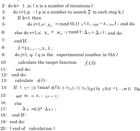
*i, β is equal to one. The controllable parameter set is searched under the satisfaction of the limiting conditions. The objective functions are calculated by a random search of controllable values with a Monte Carlo method. We have used the iterative technique instead of conventional optimal methods. This reason is to find the many pareto results to prevent the recalculation when the specification has changed. Taguchi's OA is used to consider the noise factors dealing with the production tolerance. The proposed method searches a set of design values in a direction which increases SN ratio. The bigger SN ratio gives the smaller variability from equation (2). The procedure runs in the following steps and the detail is shown in Fig.1.Step 1: Assign the noise factors to Taguchi's OA.
Step 2: In the first step, a set of controllable factors
x
ˆ
is searched from a whole range, randomly;i
x
= rand (0,1)×(x
i,high
x
i,low)
In the following steps,
x
ˆ
is selected from the range of ±Δ%, randomly .i
x
=w
i×rand ( -Δ ,Δ) ;where
w
i is the previous values ofx
i, Δ is a range width to search .Step 3: Calculate the objective functions fi(xˆ) for each experiment number of OA and each set of controllable factor
x
ˆ
.Step 4: When max ((xˆ)) is larger than the previous
0
ηunder the satisfaction of the limiting conditions,
w
iis replaced byx
iin the following step. If there was not a desirable result, the width of Δ is reduced by a half of the previous value.Step 5: Eventually, a set of controllable parameters which gives the maximum SN ratio is selected among the calculated results.
III. APPLICATION TO MICROWAVE AMPLIFIER
An input matching-circuit of a microwave amplifier is designed by the proposed method. Figure 2 shows a layout of an amplifier with FETs. The CAE model of a half of Fig.2 is illustrated in Fig.3. The input signal is divided into four circuits through the input matching-circuit and amplified by the four FET in parallel. All signals are combined with the output matching-circuit. It is important to reduce the variance of gain in order to realize the high performance. The commercial CAE code is used to calculate the performance of the circuit shown in Fig.3.
1: ( assign the noise factor s to the OA) 2: do k= 1 ,n; ( n is a number of iterations.)
3: do i=1,p ; ( p is a number to searchx in each step k.) 4: If k=1 then
5: do r=1,s ;xir = rand (0,1)×(xr,highxr,low); end do; else do r=1,s; xir= wir×rand (-Δk,+Δk end do; end If;
8: xˆ=(xi1,,xis);
9: do j=1, q; ( q is the experimental number in OA ) 10: calculate the target function fi(xˆ)
11: end do; 12 : end do;
13: calculate η(xˆ);
14: If (η=∃k(max(η(xˆ)k) >η0)∧(∀k)(gi(xˆ)k 0,(i1,,m)} Then 15: set wi xi;η0=η
16: else
17: Δk =0.5*Δk-1
18 : end If 19 : end do;
20 : ( end of calculation ) ;
; ;
6: ) ;
[image:2.595.313.550.349.571.2]7:
A. Identifying Noise and Controllable Factors
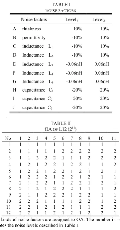
The ten kinds of noise factors and the nine kinds of controllable factors are considered in this design. The noise factors are selected and tabulated in Table I. The symbols of “A” to “J” correspond to the following; “A” and “B” are the manufacturing tolerances in the thickness and the permittivity of a base plate, respectively. “C” and “D” are the production tolerances of the inductance of lines connecting to FETs. “E” and “F” relate to the variations of inductance on the DC cut-off circuit, and “H” and “I” give the manufacturing tolerances of the capacitance of both the input and the output DC cut-off circuits. “G” is the variation of the inductance of the microstrip line connecting to the capacitor and “J” is the manufacturing tolerance of a capacitance of a bypass capacitor. Taguchi's OA is used to decrease the amount of calculations. Ten kinds of noise factors are assigned to OA of L12 (211) as shown in Table II.
The number in Table II denotes the noise levels described in Table I. The nine kinds of controllable factors are selected and they are shown in Fig.3 as the symbols enclosed in the squares. The controllable factors are three kinds of the length, L1, L2, L3, and the width, W1,W2, W3, on the
microstrip lines and the gate wire inductance, L5, connecting
to a FET. In addition, the resistace of R1 and R2 are
considered to stabilize the performance of the circuit. The manufacturing tolerances of these factors are not taken into account due to the very small production error. The FETis modeled by the measured S parameters. The calculation is done by a linear computation.
B. Calculations
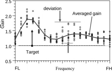
The main performance of an amplifier and its target specification is shown in Fig.4. The horizontal and vertical
axes show the frequency and the gain, respectively, where FL and FH indicate the low and high frequency within the range of use. The dotted line is the minimum of the target value. The deviation caused by the noise factors is shown in Fig. 5. The vertical line denotes the normalized gain which is expressed by the following equation (5);
10 / ) arg (
10gain T et
Gain~ (5)
[image:3.595.325.521.53.428.2]where gain is the averaged gain at each frequency. In Fig.5, the solid line indicates the averaged value and the vertical dotted symbol shows the deviation produced by the noise factors. When the gain is equal to the target value, normalized gain agrees with 1.0. Our target is to decide the FET
Fig. 2. Layout architecture of microwave amplifier.
FET Output matching-circuit L2
L1 C3 C3
C1, L3 W3,L3
W2,L2
W1, L1 R2 L4
C2, L4 L5
R1
Input matching-circuit L5
Fig. 3. Schematic drawing of CAE model. The ten kinds of noise factors and the nine kinds of the controllable factors are described in this model. The controllable factors are expressed with the symbols enclosed in the squares.
TABLEII OA OF L12(211)
No 1 2 3 4 5 6 7 8 9 10 11
1 1 1 1 1 1 1 1 1 1 1 1
2 1 1 1 1 1 2 2 2 2 2 2
3 1 1 2 2 2 1 1 1 2 2 2
4 1 2 1 2 2 1 2 2 1 1 2
5 1 2 2 1 2 2 1 2 1 2 1
6 1 2 2 2 1 2 2 1 2 1 1
7 2 1 2 2 1 1 2 2 1 2 1
8 2 1 2 1 2 2 2 1 1 1 2
9 2 1 1 2 2 2 1 2 2 1 1
10 2 2 2 1 1 1 1 2 2 1 2
11 2 2 1 2 1 2 1 1 1 2 2
12 2 2 1 1 2 1 2 1 2 2 1
Ten kinds of noise factors are assigned to OA. The number in matrix denotes the noise levels described in Table I
Gai
n
(
d
B
)
FL FH
5 10
0 15
Target
Design region
[image:3.595.68.291.55.150.2]Frequency
Fig. 4. The main performance of an amplifier and its target. The dotted line is a minimum of a target value.
TABLEI NOISE FACTORS
Noise factors Level1 Level2
A thickness -10% 10%
B permittivity -10% 10%
C inductance L1 -10% 10%
D Inductance L2 -10% 10%
E inductance L3 -0.06nH 0.06nH F Inductance L4 -0.06nH 0.06nH G Inductance L5 -0.06nH 0.06nH
H capacitance C1 -20% 20%
I capacitance C2 -20% 20%
J capacitance C3 -20% 20%
[image:3.595.53.285.178.306.2] [image:3.595.322.525.441.577.2]values of controllable factors which can make the deviation from averaged gain smaller. The stabilization coefficient of this amplifier is also considered as a condition of the limitation.
[image:4.595.316.521.63.217.2]IV. RESULTS AND DISCUSSIONNS
Fig.6 shows the calculated results. The horizontal line gives the SN Ratio,η, and the vertical line shows the minimum value of Gain~ . The 100 points are plotted for each of ten iterations. In the first step, the initial value is decided with the uniform random search in the whole range of controllable factors. In the second step, the range width is set as Δ=50%. In the following steps, Δ is changed with the range width shown in Fig.7. From Fig.6, the calculated results gradually converge to the value which gives a larger SN ratio. The proposed method is also compared with the results described by the symbol of ●, which are calculated
by SA algorithm. The proposed method searches the pareto front. It also shows that ηhas a tradeoff toward a gain. Fig.7 shows the relationship between ηand the number of iterations. The horizontal line denotes the number of iterations. The vertical lines show the η and Δ. ηincreases from 35.8 db in the initial step to 43.1 db in the final result. This means that the variation decreased to a 0.43 of an initial value expressed with the coefficient of variation. The calculation is converged by 10 iterations. CPU time is 360 sec with Intel Core i5-2500 processor in a Windows PC. Although the number of calculated points is 100 on each iteration step, the designer can change it depending on the distribution of results.
Fig.8 shows the frequency response of gain at the design points “A” ~”D” shown in Fig.6. “A” and “D” give the minimum and the maximum of SN ratios in Fig.6. “B” gives the maximum gain, and “C”shows the final design. Fig.8 shows that the larger SN ratio gives the smaller variance of the gain. The design “C” is selected to achieve the target value even if the worst case production occurred.
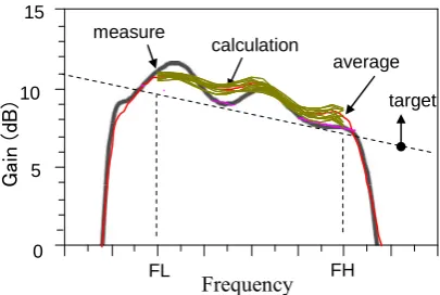
The initial configuration was modified under the limitation on the substrate size. The response of the circuit was confirmed by the electromagnetic field computation, and it was tuned to avoid the undesirable oscillations. We have manufactured the prototype amplifier based on this result. The frequency response of the prototype is compared with the calculation in Fig.9. In Fig.9, the bold line shows the measurement and the flux of thin lines are the calculations which include the variance caused by the noise
factors. The calculated result agrees with the measurement qualitatively, and the gain satisfies the specification.
0.6 0.7 0.8 0.9 1 1.1 1.2 1.3
35 36 37 38 39 40 41 42 43 44
η (db)
mi
n
(G
a
in
)
~
B
C
[image:4.595.65.257.113.236.2]A D
Fig. 6. Calculated results. The 100 points are plotted for each of ten iterations. In the first step, the initial value is decided by the random search in the design space. In the following steps, the scale ranges are decreased by the half of the previous ones.
30 32 34 36 38 40 42 44
1 6 11 16
Number of Iteration
SN rati
o
η
0 10 20 30 40 50 60
R
an
ge
w
idth
Δ
(%)
[image:4.595.325.533.272.419.2]10th iteration
Fig. 7. The relationship between SN ratio, η, and range width, Δ, corresponding to the number of iteration.
Ga
in
FL FH
1.0 1.5 2.0
0.5 2.5
Averaged gain
Target
deviation
Frequency
~
Fig. 5. The main performance of the amplifier and its targeted value. The vertical line denotes the normalized gain.
0 2 4 6 8 10 12 14 16
Ga
in
(d
B
)
FL Frequency FH
2 4 6 8 10 12 14
0 16
Ga
in
(d
B)
FL Frequency FH (a) design points A (b) design points B
2 4 6 8 10 12 14
0 16
2 4 6 8 10 12 14
0 16
FL Frequency FH
Ga
in
(d
B
)
FL Frequency FH
Gain (dB)
[image:4.595.313.551.455.643.2]The experimental gain in the mass production is plotted in Fig.10. The maximum and the minimum value correspond to the minimum and the maximum gain in all experiments, respectively. The average gain was ±0.6 dB and the standard deviation was 0.2 dB. The first run rate obtained 97 %.
V. CONCLUSION
A useful robust parameter design methodology is proposed for a microwave circuit. A set of design values is decided to satisfy the specification and to reduce the variability of the performance in the manufacture. The multi-objective problem is treated as a single optimization problem. The function which shows the variability of the ideal relationship between signal and response is minimized under the limiting conditions based on the specifications. The proposed method is applied to the design of a microwave amplifier, and its effectiveness is studied with the CAE simulation and the experiments. It results that the first run rate achieved 97 % in the manufactures.
REFERENCES
[1] Shuich. Ota, Reliability Engineering Association of Japan (REAJ), Vol.25, No.8, 2003, pp.865 -868, (in Japanese)
[2] N. Shigyo H. Tanimoto T. Morishita K. Sugawara N. Wakita Y, Asahi, “Statistical simulation of MOSFETs using TCAD: meshing noise problem and selection of factors,” 3rd International Workshop on Statistical Metrology, 1998, pp10-13
[3] Stephen W., Peter Feldmann and Kannan Krishna, “Statistical Integrated Circuit Design,“ IEEE Journal of Solid-State Circuits, Vol. 28. No. 3, 1993, pp.193-202
[4] Norman J. Elias,” Acceptance Sampling: An Efficient, “Accurate Method for Estimating and Optimizing Parametric Yield,” IEEE Journal of Solid-Stats,. Vol. 29. No. 3, 1994, pp323-327
[5] Ricardo S. Zebulum , Marco Aurélio Pacheco and Marley Vellasco, “A Multi-Objective Optimization Methodology Applied to the Synthesis of Low-Power Operational Amplifiers,” Proceedings of the XIII International Conference in Microelectronics and Packaging,
Vol.1.,1998, pp.264-271
[6] Leonard0 C. Brito and Paul0 H. P. de Carvalho, “_An evolutionary approach for multi-objective optimization of nonlinear microwave circuits,” IEEE MTT-S International Microwave Symposium Digest, Vol.2 , 2004, pp949-952
[7] Eckart Zitzler and Lothar Thiele, “Multiobjective Evolutionary Algorithms: A Comparative Case Study and the Strength Pareto Approach,” IEEE Transactions on evolutionary Computation, Vol. 3, No. 4, 1994, pp257-271
[8] Lingling Sun, Zhi Zhou, Xungen Li and Wenming Zhao, “A new optimization method for microwave broad band amplifier based on orthogonal design,” Proceedings. 6th International Conference on Solid-State and Integrated-Circuit Technology, 2001, pp1151-1154 [9] Hiroyuki KAWAGISHI and Kazuhiko KUDO, “Development of
Grobal Optimization Method by Orthogonal Array (Application to Mechanical Design Problem),” The Japan Society of Mechanical Engineering, 2007, pp2335-2342
[10] Fatemeh Kashfi, Safar Hatami and Massoud Pedram,
“Multi-objective optimization techniques for VLSI circuits, “ IEEE 12th International Symposium on Quality Electronic Design, 2011, pp156-163
[11] KUROIWA Tadashi, “Trade-off Analysis Method,” TOSHIBA Review Vol.60, No.1, 2005, pp48-51 (in Japanese)
[12] Satoshi KITAYAMA, Koetsu YAMAZAKI, Masao ARAKAWA, and Hiroshi YAMAKAWA, “Trade-Off Analysis on the Multi-Objective Design Optimization,” Transactions of the Japan Society of Mechanical Engineers, Part C, 75(754), 2009, pp1828-1836, (in Japanese)
[13] Sawal Ali, Beuben Wilcock, Peter Wilson and Anderew Brown, “Yield Model Characterization for Analog Integrated Circuit Using Pareto-Optimal Surface,” IEEE International Conference on Electronics, Circuits, and Systems, 2008
[14] Genichi Taguchi, “ Taguchi methods in LSI fabrication process,” 6th International Workshop on Statistical Methodology, 2001, pp.1-6 [15] Genichi Taguchi and Shih-Chung Tsai, ”Quality Engineering
(Taguchi Methods). For The Development of Electronic Circuit Technology,” IEEE Transactions on Reliability, Vol.44, N0.2, 1995, pp225-229
[16] R. D. Kulkarni and Vivek Agarwal, ” Taguchi Based Performance and Reliability. Improvement of an Ion Chamber Amplifier for Enhanced Nuclear Reactor Safety,” IEEE Transactions on Nuclear Science, Vol.55, No.4, 2008, pp2303-2313
[17] Kun-Lin Hsieh, Lee-Ing Tong Hung-Pin Chiu and Hsin-Ya Yeh, “Optimization of a multi-response problem in Taguchi’s dynamic system,” Computers & Industrial Engineering Vol.49, 2005, pp.556–571
[18] Lee-Ing Tong a, Chung-Ho Wang, Chih-Chien Chen and Chun-Tzu Chen, “Dynamic multiple responses by ideal solution analysis”,
European Journal of Operational Research, Vol..56, No.16, 2004, pp433–444
[19] Hsu-Hwa Chang, “A data mining approach to dynamic multiple responses in Taguchi experimental Design,” Expert Systems with Applications, Vol. 35, 2008, pp.1095-1103
[20] V N Gaitondea,S R Karnikb, B T Achyuthac and B Siddeswarappad, “Multi-response optimization in drilling using Taguchi's quality loss function,” Indian Journal of Engineering & Materials Sciences, Vol. 13; No. 6, 2006, pp. 484-48
[21] Ful-Chiang Wu; Bing-Chang Ouyang, Cheng-Hsiung Chen and Chi-Hao Yeh, “Robust design of nonlinear dynamic problem,” 2010 2nd International Conference on Education Technology and Computer (ICETC), 2010, pp.V1-162 -166
[22] Jim Carroll and K and Ghang, “Statistical Computer- Aided Design for Microwave Circuits,” IEEE Transactions on Microwaves and Technology, Vol.44, No.1, 1992, pp.24-32
[23] Young, D.L., Teplik, J., Weed, H.D., Tracht, N.T. and Alvarez, A.R., “Application of statistical design and response surface methods to computer-aided VLSI device design II. Desirability functions and Taguchi methods,” IEEE Transactions on Computer-Aided Design of Integrated Circuits and Systems, Vol.10, 1991, pp.103-115
[24] Ming-Ru Chen , “Robust design for VLSI process and device,” 6th International Workshop on Statistical Methodology, 2001, pp.7-16 Fig. 10. Normalized gain obtained by the experiments in the
manufactures.
FL FH
5 10
0 15
calculation measure
target
Gai
n (d
B
)
Frequency
average
[image:5.595.57.268.328.432.2][25] Pisvimol Chatsirirungruang, “Application of Computer Aided Engineering with Genetic Algorithm and Taguchi method in Nonlinear Double-Dynamic Robust Parameter Design,” Proceedings of the International MultiConference of Engineers and Computer Scientists, 2010, pp.17-19
[26] Pisvimol Chatsirirungruang and Masami Miyakawa ,“Application of genetic algorithm to numerical experiment in robust parameter design for signal multi-response problem, “ Journal of Management Science and Engineering Management, Vol.4 No.1, 2009, pp.49-59 [27] Nakayama, H., “Proposal of Satisfying Trade-Off Method for
Multiobjective Programming, “ Journal of the Society of Instrument and Control Engineers, Vol.20, No.1, 1984, pp.29-35 (in Japanese) [28] Ful-Chiang Wu, Bing-Chang Ouyang, Cheng-Hsiung Chen and