Incorporating Glosses into Neural Word Sense Disambiguation

2473

Incorporating Glosses into Neural Word Sense Disambiguation

Fuli Luo, Tianyu Liu, Qiaolin Xia, Baobao Chang and Zhifang Sui Key Laboratory of Computational Linguistics, Ministry of Education,

School of Electronics Engineering and Computer Science, Peking University, Beijing, China {luofuli, tianyu0421, xql, chbb, szf}@pku.edu.cn

Abstract

Word Sense Disambiguation (WSD) aims to identify the correct meaning of poly-semous words in the particular context. Lexical resources like WordNet which are proved to be of great help for WSD in the knowledge-based methods. However, previous neural networks for WSD always rely on massive labeled data (context), ig-noring lexical resources like glosses (sense definitions). In this paper, we integrate the context and glosses of the target word into a unified framework in order to make full use of both labeled data and lexi-cal knowledge. Therefore, we propose

GAS: agloss-augmented WSD neural net-work which jointly encodes the context and glosses of the target word. GAS mod-els the semantic relationship between the context and the gloss in an improved mem-ory network framework, which breaks the barriers of the previous supervised methods and knowledge-based methods. We further extend the original gloss of word sense via its semantic relations in WordNet to enrich the gloss informa-tion. The experimental results show that our model outperforms the state-of-the-art systems on several English all-words WSD datasets.

1 Introduction

Word Sense Disambiguation (WSD) is a funda-mental task and long-standing challenge in Nat-ural Language Processing (NLP). There are sev-eral lines of research on WSD. Knowledge-based methods focus on exploiting lexical resources to infer the senses of word in the context. Super-vised methods usually train multiple classifiers

with manual designed features. Although suvised methods can achieve the state-of-the-art per-formance (Raganato et al.,2017b,a), there are still two major challenges.

Firstly, supervised methods (Zhi and Ng,2010; Iacobacci et al., 2016) usually train a dedicated classifier for each word individually (often called

word expert). So it can not easily scale up to

all-words WSD task which requires to disam-biguate all the polysemous word in texts1. Recent neural-based methods (K˚ageb¨ack and Salomons-son,2016;Raganato et al.,2017a) solve this prob-lem by building a unified model for all the polyse-mous words, but they still can’t beat the bestword

expertsystem.

Secondly, all the neural-based methods always only consider the local context of the target word, ignoring the lexical resources like Word-Net (Miller, 1995) which are widely used in the knowledge-based methods. The gloss, which ex-tensionally defines a word sense meaning, plays a key role in the well-known Lesk algorithm (Lesk, 1986). Recent studies (Banerjee and Pedersen, 2002;Basile et al.,2014) have shown that enrich-ing gloss information through its semantic rela-tions can greatly improve the accuracy of Lesk al-gorithm.

To this end, our goal is to incorporate the gloss information into a unified neural network for all of the polysemous words. We further consider ex-tending the original gloss through its semantic re-lations in our framework. As shown in Figure1, the glosses of hypernyms and hyponyms can en-rich the original gloss information as well as help to build better a sense representation. Therefore, we integrate not only the original gloss but also the related glosses of hypernyms and hyponyms into the neural network.

bed2

Original gloss

a plot of ground in which plants are growing

a small area of ground covered by specific vegetation

flowerbed1

a bed in which

flowers are growing

seedbed1

a bed where seedlings are grown before transplanting

turnip_bed1

a bed in which

turnips are growing

Example sentence

the gardener planted a bed of roses

H

yp

er

n

ym

y

H

yp

o

n

ym

y

plot2

Figure 1: The hypernym (green node) and hy-ponyms (blue nodes) for the 2nd sense bed2 of bed, which meansa plot of ground in which plants

are growing, rather than the bed for sleeping in.

The figure shows thatbed2 is a kind ofplot2, and

bed2includesf lowerbed1,seedbed1, etc.

In this paper, we propose a novel modelGAS: a

gloss-augmented WSD neural network which is a variant of the memory network (Sukhbaatar et al., 2015b; Kumar et al., 2016; Xiong et al., 2016). GAS jointly encodes the context and glosses of the target word and models the semantic relationship between the context and glosses in the memory module. In order to measure the inner relationship between glosses and context more accurately, we employ multiple passes operation within the ory as the re-reading process and adopt two mem-ory updating mechanisms.

The main contributions of this paper are listed as follows:

• To the best of our knowledge, our model is the first to incorporate the glosses into an end-to-end neural WSD model. In this way, our model can benefit from not only massive labeled data but also rich lexical knowledge.

• In order to model semantic relationship of context and glosses, we propose a gloss-augmented neural network (GAS) in an im-proved memory network paradigm.

• We further expand the gloss through its se-mantic relations to enrich the gloss informa-tion and better infer the context. We extend the gloss module in GAS to a hierarchical framework in order to mirror the hierarchies of word senses in WordNet.

• The experimental results on several English all-words WSD benchmark datasets show that our model outperforms the state-of-the-art systems.

2 Related Work

Knowledge-based, supervised and neural-based methods have already been applied to WSD task (Navigli,2009).

Knowledge-based WSD methods mainly ex-ploit two kinds of knowledge to disambiguate pol-ysemous words: 1) The gloss, which defines a word sense meaning, is mainly used in Lesk al-gorithm (Lesk, 1986) and its variants. 2) The structure of the semantic network, whose nodes are synsets 2 and edges are semantic relations, is mainly used in graph-based algorithms (Agirre et al.,2014;Moro et al.,2014).

Supervised methods (Zhi and Ng, 2010; Ia-cobacci et al., 2016) usually involve each target word as a separate classification problem (often calledword expert) and train classifiers based on manual designed features.

Although word expert supervised WSD meth-ods perform best in terms of accuray, they are less flexible than knowledge-based methods in the all-words WSD task (Raganato et al., 2017a). To deal with this problem, recent neural-based meth-ods aim to build a unified classifier which shares parameters among all the polysemous words. K˚ageb¨ack and Salomonsson(2016) leverages the bidirectional long short-term memory network which shares model parameters among all the pol-ysemous words. Raganato et al.(2017a) transfers the WSD problem into a neural sequence labeling task. However, none of the neural-based methods can totally beat the best word expert supervised methods on English all-words WSD datasets.

What’s more, all of the previous supervised methods and neural-based methods rarely take the lexical resources like WordNet (Fellbaum, 1998) into consideration. Recent studies on sense em-beddings have proved that lexical resources are helpful. Chen et al. (2015) trains word sense embeddings through learning sentence level em-beddings from glosses using a convolutional neu-ral networks. Rothe and Sch¨utze(2015) extends word embeddings to sense embeddings by using the constraints and semantic relations in WordNet. They achieve an improvement of more than 1% in WSD performance when using sense embed-dings as WSD features for SVM classifier. This work shows that integrating structural information of lexical resources can help to word expert su-pervised methods. However, sense embeddings

can only indirectly help to WSD (as SVM clas-sifier features).Raganato et al.(2017a) shows that the coarse-grained semantic labels in WordNet can help to WSD in a multi-task learning framework. As far as we know, there is no study directly inte-grates glosses or semantic relations of the Word-Net into an end-to-end model.

In this paper, we focus on how to integrate glosses into a unified neural WSD system. Mem-ory network (Sukhbaatar et al., 2015b; Kumar et al., 2016; Xiong et al., 2016) is initially pro-posed to solve question answering problems. Re-cent researches show that memory network ob-tains the state-of-the-art results in many NLP tasks such as sentiment classification (Li et al., 2017) and analysis (Gui et al.,2017), poetry generation (Zhang et al.,2017), spoken language understand-ing (Chen et al.,2016), etc. Inspired by the suc-cess of memory network used in many NLP tasks, we introduce it into WSD. We make some adap-tations to the initial memory network in order to incorporate glosses and capture the inner relation-ship between the context and glosses.

3 Incorporating Glosses into Neural Word Sense Disambiguation

In this section, we first give an overview of the proposed model GAS: a gloss-augmented WSD neural network which integrates the context and the glosses of the target word into a unified frame-work. After that, each individual module is de-scribed in detail.

3.1 Architecture of GAS

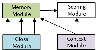
The overall architecture of the proposed model is shown in Figure2. It consists of four modules:

• Context Module: The context module en-codes the local context (a sequence of sur-rounding words) of the target word into a dis-tributed vector representation.

• Gloss Module: Like the context module, the gloss module encodes all the glosses of the target word into a separate vector representa-tions of the same size. In other words, we can get|st|word sense representations according to|st|3senses of the target word, where|st| is the sense number of the target wordwt.

3_s

tis the sense set{s1t, s2t, . . . , s p

t}corresponding to the target wordxt

Gloss Module

Context Module Memory

Module

Scoring Module

Figure 2: Overview of Gloss-augmented Memory Network for Word Sense Disambiguation.

• Memory Module: The memory module is employed to model the semantic relationship between the context embedding and gloss embedding produced by context module and gloss module respectively.

• Scoring Module: In order to benefit from both labeled contexts and gloss knowledge, the scoring module takes the context embed-ding from context module and the last step result from the memory module as input. Fi-nally it generates a probability distribution over all the possible senses of the target word.

Detailed architecture of the proposed model is shown in Figure 3. The next four sections will show detailed configurations in each module.

3.2 Context Module

Context module encodes the context of the target word into a vector representation, which is also called context embedding in this paper.

We leverage the bidirectional long short-term memory network (Bi-LSTM) for taking both the preceding and following words of the target word into consideration. The input of this mod-ule [x1, . . . , xt−1, xt+1, . . . , xTx] is a sequence of words surrounding the target word xt, where

Tx is the length of the context. After apply-ing a lookup operation over the pre-trained word embedding matrix M ∈ _RD×V_{, we transfer a} one hot vector xi into a D-dimensional vec-tor. Then, the forward LSTM reads the segment

(x1, . . . , xt−1) on the left of the target word xt

and calculates a sequence offorward hidden states (−→h1, . . . ,

− →

ht−1). The backward LSTM reads the segment (xTx, . . . , xt+1) on the right of the tar-get wordxtand calculates a sequence ofbackward hidden states(←−hTx, . . . ,

←−

ht+1). The context vec-torcis finally concatenated as

c= [−→ht−1 :

←−

Scoring Module

Gloss Module Gloss

Reader Layer h-K

Relation Fusion Layer

h0

h0 h+1 h+K

x 10

0 hG g-1

g-K g+1 g+K

hypernyms hyponyms

h-1

x 20 _{x G}0 h10

Context Module

x 1 x t-1 x T

ht+1 Memory

Module m2

m1 _W

+ scoreg

scorec

ht-1

x t-1

i i i i

g1 g2 g3

GAS

GAS

g0i g0i

r_i r_i

Original Gloss

Extended Glosses

g

Figure 3: Detailed architecture of our proposed model, which consists of a context module, a gloss module, a memory module and a scoring module. The context module encodes the adjacent words surrounding the target word into a vectorc. The gloss module encodes the original gloss or extended glosses into a vectorgi. In the memory module, we calculate the inner relationship (as attention) between contextcand each glossgiand then update the memory asmiat passi. In the scoring module, we make final predictions based on the last pass attention of memory module and the context vector c. Note that GAS only uses the original gloss, while GASextuses the entended glosses through hypernymy and hyponymy relations. In other words, the relation fusion layer (grey dotted box) only belongs to GASext.

where:is the concatenation operator.

3.3 Gloss Module

The gloss module encodes each gloss of the target word into a fixed size vector like the context vec-tor c, which is also called gloss embedding. We further enrich the gloss information by taking se-mantic relations and their associated glosses into consideration.

This module contains a gloss reader layer and a relation fusion layer. Gloss reader layer gener-ates a vector representations for a gloss. Relation fusion layer aims at modeling the semantic rela-tions of each gloss in the expanded glosses list which consists of related glosses of the original gloss. Our model GAS with extended glosses is denoted as GASext. GAS only encodes the orig-inal gloss, while GASext encodes the expanded glosses from hypernymy and hyponymy relations (details in Figure3).

3.3.1 Gloss Reader Layer

Gloss reader layer contains two parts: gloss ex-pansion and gloss encoder. Gloss exex-pansion is to enrich the original gloss information through its

hypernymy and hyponymy relations in WordNet. Gloss encoder is to encode each gloss into a vec-tor representation.

Gloss Expansion: We only expand the glosses of nouns and verbs via their corresponding hyper-nyms and hypohyper-nyms. There are two reasons: One is that most of polysemous words (about 80%) are nouns and verbs; the other is that the most frequent relations among word senses for nouns and verbs are the hypernymy and hyponymy relations4.

The original gloss is denoted as g0. Breadth-first search method with a limited depth K is employed to extract the related glosses. The glosses of hypernyms within K depth are de-noted as [g−1, g−2, . . . , g−L1]. The glosses of hyponyms within K depth are denoted as

[g+1, g+2, . . . , g+L2]5. Note thatg+1andg−1are the glosses of the nearest word sense.

Gloss Encoder: We denote thej-th 6 gloss in

4

In WordNet, more than 95% of relations for nouns and 80% for verbs are hypernymy and hyponymy relations.

5

Since one synset has one or more direct hypernyms and hyponyms,L1>=KandL2 >=K.

6_{Since GAS don’t have gloss expansion, j is always 0 and} gi= gi

the expanded glosses list forithsense of the target word as a sequence of G words. Like the con-text encoder, the gloss encoder also leverages Bi-LSTM units to process the words sequence of the gloss. The gloss representationgi_j is computed as the concatenation of the last hidden states of the

forwardandbackwardLSTM.

g_ji = [−→h_Gi,j :←−hi,j₁ ] (2)

where j ∈ [−L1, . . . ,−1,0,+1, . . . ,+L2]and : is the concatenation operator .

3.3.2 Relation Fusion Layer

Relation fusion layer models the hypernymy and hyponymy relations of the target word sense. A forward LSTM is employed to encode the hypernyms’ glosses of ith sense

(gi

−L1, . . . , gi−1, gi0) as a sequence of forward

hidden states (−→hi_−L1, . . . ,−→hi₋₁,−→hi₀). A back-ward LSTM is employed to encode the hy-ponyms’ glosses of ith sense (g+iL2, . . . , gi+1, g0i) as a sequence of backward hidden states (←−hi_+L2, . . . ,←h−i₊₁,←−hi₀). In order to highlight the original glossg₀i, the enhancedithsense represen-tation is concatenated as the final state of the for-ward and backfor-ward LSTM.

gi = [

− →

hi₀ :←−hi₀] (3)

3.4 Memory Module

The memory module has two inputs: the context vector c from the context module and the gloss vectors{g1, g2, . . . , g|st|} from the gloss module, where |st| is the number of word senses. We model the inner relationship between the context and glosses by attention calculation. Since one-pass attention calculation may not fully reflect the relationship between the context and glosses (de-tails in Section4.4.2), the memory module adopts a repeated deliberation process. The process re-peats reading gloss vectors in the following passes, in order to highlight the correct word sense for the following scoring module by a more accurate at-tention calculation. After each pass, we update the memory to refine the states of the current pass. Therefore, memory module contains two phases: attention calculation and memory update.

Attention Calculation: For each passk, the at-tentionek_i of glossgiis generally computed as

ek_i =f(gi, mk−1, c) (4)

wheremk−1 is the memory vector in the(k−1) -th pass while c is the context vector. The scor-ing function f calculates the semantic relation-ship of the gloss and context, taking the vector set(gi, mk−1, c)as input. In the first pass, the at-tention reflects the similarity of context and each gloss. In the next pass, the attention reflects the similarity of adapted memory and each gloss. A dot product is applied to calculate the similarity of each gloss vector and context (or memory) vector. We treatcasm0. So, the attentionαk_i of glossgi at passk is computed as a dot product ofgi and

mk−1:

ek_i =gi·mk−1 (5)

αk_i = exp(e

k i)

P|st| j=1exp(e

j i)

(6)

Memory Update: After calculating the atten-tion, we store the memory state inuk which is a weighted sum of gloss vectors and is computed as

uk=

n

X

i=1

αk_igi (7)

where nis the hidden size of LSTM in the con-text module and gloss module. And then, we up-date the memory vectormkfrom last pass memory

mk−1, context vectorc, and memory stateuk. We propose two memory update methods:

• Linear: we update the memory vectormkby

a linear transformation frommk−1

mk =Hmk−1+uk (8)

whereH∈_R2n×2n_.

• Concatenation: we get a new memory fork

-th pass by taking bo-th -the gloss embedding and context embedding into consideration

mk=ReLU(W[mk−1 :uk :c] +b) (9)

where:is the concatenation operator, W ∈ Rn×6nandb∈R2n.

3.5 Scoring Module

The scoring module calculates the scores for all the related senses {s1_t, s2_t, . . . , sp_t} corresponding to the target word xt and finally outputs a sense probability distribution over all senses.

The overall score for each word sense is deter-mined by gloss attention αTM

in the memory module, whereTM is the number of passes in the memory module. TheeTM _(αTM without Softmax) is regarded as the gloss score.

scoreg =eTM (10)

Meanwhile, a fully-connected layer is em-ployed to calculate the context score.

scorec=Wxtc+bxt (11)

where Wxt ∈R

|st|×2n_{, b}

xt ∈ R

|st|_{, |s}

t| is the number of senses for the target wordxtandnis the number of hidden units in the LSTM.

It’s noteworthy that in Equation 11, each am-biguous wordxthas its corresponding weight ma-trixWxt and biasbxtin the scoring module.

In order to balance the importance of back-ground knowledge and labeled data, we introduce a parameter λ ∈ _RN 7 _{in the scoring module} which is jointly learned during the training pro-cess. The probability distribution yˆ over all the word senses of the target word is calculated as:

ˆ

y=Sof tmax(λxtscorec+ (1−λxt)scoreg)

where λxt is the parameter for word xt, and

λxt ∈[0,1].

During training, all model parameters are jointly learned by minimizing a standard cross-entropy loss betweenyˆand the true labely.

4 Experiments and Evaluation

4.1 Dataset

Evaluation Dataset: we evaluate our model on several English all-words WSD datasets. For fair comparison, we use the benchmark datasets proposed by Raganato et al. (2017b) which in-cludes five standard all-words fine-grained WSD datasets from the Senseval and SemEval competi-tions. They are Senseval-2 (SE2), Senseval-3 task 1 (SE3), SemEval-07 task 17 (SE7), SemEval-13 task 12 (SE13), and SemEval-15 task 13 (SE15). Following byRaganato et al.(2017a), we choose SE7, the smallest test set as the development (val-idation) set, which consists of 455 labeled in-stances. The last four test sets consist of 6798 labeled instances with four types of target words, namely nouns, verbs, adverbs and adjectives. We

7_{N is the number of polysemous words in the training} corpora.

extract word sense glosses from WordNet3.0 be-cause Raganato et al.(2017b) maps all the sense annotations8from its original version to 3.0.

Training Dataset: We choose SemCor 3.0 as the training set, which was also used byRaganato et al.(2017a),Raganato et al.(2017b),Iacobacci et al.(2016),Zhi and Ng(2010), etc. It consists of 226,036 sense annotations from 352 documents, which is the largest manually annotated corpus for WSD. Note that all the systems listed in Table1 are trained on SemCor 3.0.

4.2 Implementation Details

We use the validation set (SE7) to find the optimal settings of our framework: the hidden state size

n, the number of passes|TM|, the optimizer, etc. We use pre-trained word embeddings with 300 di-mensions9, and keep them fixed during the train-ing process. We employ 256 hidden units in both the gloss module and the context module, which meansn=256. Orthogonal initialization is used for weights in LSTM and random uniform initializa-tion with range [-0.1, 0.1] is used for others. We assign gloss expansion depthKthe value of 4. We also experiment with the number of passes|TM| from 1 to 5 in our framework, finding|TM| =3 performs best. We use Adam optimizer (Kingma and Ba, 2014) in the training process with 0.001 initial learning rate. In order to avoid overfitting, we use dropout regularization and set drop rate to 0.5. Training runs for up to 100 epochs with early stopping if the validation loss doesn’t im-prove within the last 10 epochs.

4.3 Systems to be Compared

In this section, we describe several knowledge-based methods, supervised methods and neural-based methods which perform well on the English all-words WSD datasets for comparison.

4.3.1 Knowledge-based Systems

• Leskext+emb: Basile et al.(2014) is a vari-ant of Lesk algorithm (Lesk, 1986) by us-ing a word similarity function defined on a distributional semantic space to calculate the gloss-context overlap. This work shows that glosses are important to WSD and enriching

8_{The original WordNet version of SE2, SE3, SE7, SE13,} SE15 are 1.7, 1.7.1, 2.1, 3.0 and 3.0, respectively.

9_{We download the pre-trained word embeddings from}

Test Datasets Concatenation of Test Datasets

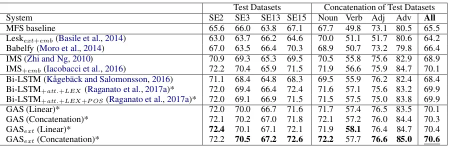
System SE2 SE3 SE13 SE15 Noun Verb Adj Adv All

MFS baseline 65.6 66.0 63.8 67.1 67.7 49.8 73.1 80.5 65.5

Leskext+emb(Basile et al.,2014) 63.0 63.7 66.2 64.6 70.0 51.1 51.7 80.6 64.2

Babelfy (Moro et al.,2014) 67.0 63.5 66.4 70.3 68.9 50.7 73.2 79.8 66.4

IMS (Zhi and Ng,2010) 70.9 69.3 65.3 69.5 70.5 55.8 75.6 82.9 68.9

IMS+emb(Iacobacci et al.,2016) 72.2 70.4 65.9 71.5 71.9 56.6 75.9 84.7 70.1 Bi-LSTM (K˚ageb¨ack and Salomonsson,2016) 71.1 68.4 64.8 68.3 69.5 55.9 76.2 82.4 68.4 Bi-LSTM+att.+LEX(Raganato et al.,2017a)* 72.0 69.4 66.4 72.4 71.6 57.1 75.6 83.2 69.9 Bi-LSTM+att.+LEX+P OS(Raganato et al.,2017a)* 72.0 69.1 66.9 71.5 71.5 57.5 75.0 83.8 69.9

GAS (Linear)* 72.0 70.0 66.7 71.6 71.7 57.4 76.5 83.5 70.1

GAS (Concatenation)* 72.1 70.2 67.0 71.8 72.1 57.2 76.0 84.4 70.3

GASext(Linear)* 72.4 70.1 67.1 72.1 71.9 58.1 76.4 84.7 70.4

GASext(Concatenation)* 72.2 70.5 67.2 72.6 72.2 57.7 76.6 85.0 70.6

Table 1: F1-score (%) for fine-grained English all-words WSD on the test sets. Boldfont indicates best systems. The * represents the neural network models using external knowledge. The fives blocks list the MFS baseline, two knowledge-based systems, two supervised systems (feature-based), three neural-based systems and our models, respectively.

.

gloss information via its semantic relations can help to WSD.

• Babelfy: Moro et al. (2014) exploits the se-mantic network structure from BabelNet and builds a unified graph-based architecture for WSD and Entity Linking.

4.3.2 Supervised Systems

The supervised systems mentioned in this paper refers to traditional feature-based systems which train a dedicated classifier for every word individ-ually (word expert).

• IMS:Zhi and Ng(2010) selects a linear Sup-port Vector Machine (SVM) as its classifier and makes use of a set of features surround-ing the target word within a limited window, such as POS tags, local words and local col-locations.

• IMS+emb: Iacobacci et al. (2016) selects IMS as the underlying framework and makes use of word embeddings as features which makes it hard to beat in most of WSD datasets.

4.3.3 Neural-based Systems

Neural-based systems aim to build an end-to-end unified neural network for all the polysemous words in texts.

• Bi-LSTM: K˚ageb¨ack and Salomonsson (2016) leverages a bidirectional LSTM network which shares model parameters among all words. Note that this model is equivalent to our model if we remove the gloss module and memory module of GAS.

• Bi-LSTM+att.+LEX and its variant

Bi-LSTM+att.+LEX+P OS: Raganato et al. (2017a) transfers WSD into a sequence ing task and propose a multi-task learn-ing framework for WSD, POS tagglearn-ing and coarse-grained semantic labels (LEX). These two models have used the external knowl-edge, for the LEX is based on lexicographer files in WordNet.

Moreover, we introduce MFSbaseline, which simply selects the most frequent sense in the train-ing data set.

4.4 Results and Discussion

4.4.1 English all-words results

In this section, we show the performance of our proposed model in the English all-words task. Ta-ble 1 shows the F1-score results on the four test sets mentioned in Section 4.1. The systems in the first four blocks are implemented byRaganato et al. (2017a,b) except for the single Bi-LSTM model. The last block lists the performance of our proposed model GAS and its variant GASext which extends the gloss module in GAS.

GAS and GASext achieves the state-of-the-art performance on the concatenation of all test datasets. Although there is no one system al-ways performs best on all the test sets10, we can find that GASextwithconcatenationmemory up-dating strategy achieves the best results 70.6 on the concatenation of the four test datasets. Com-pared with other three neural-based methods in the

Context: Heplaysa pianist in the film

Glosses Pass 1 Pass 2 Pass 3 Pass 4 Pass 5

g1: participate in games or sport

g2: perform music on a instrument

g3: act a role or part

Table 2: An example of attention weights in the memory module within 5 passes. Darker colors mean that the attention weight is higher. Case studies show that the proposed multi-pass operation can recognize the correct sense by enlarging the attention gap between correct senses and incorrect ones.

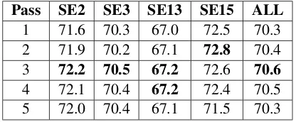
Pass SE2 SE3 SE13 SE15 ALL

1 71.6 70.3 67.0 72.5 70.3

2 71.9 70.2 67.1 72.8 70.4

3 72.2 70.5 67.2 72.6 70.6

4 72.1 70.4 67.2 72.4 70.5

5 72.0 70.4 67.1 71.5 70.3

Table 3: F1-score (%) of different passes from 1 to 5 on the test data sets. It shows that appropri-ate number of passes can boost the performance as well as avoid over-fitting of the model.

.

fourth block, we can find that our best model out-performs the previous best neural network models (Raganato et al., 2017a) on every individual test set. The IMS+emb, which trains a dedicated classi-fier for each word individually (word expert) with massive manual designed features including word embeddings, is hard to beat for neural networks models. However, our best model can also beat IMS+embon the SE3, SE13 and SE15 test sets.

Incorporating glosses into neural WSD can greatly improve the performance and extending the original gloss can further boost the results. Compared with the Bi-LSTM baseline which only uses labeled data, our proposed model greatly im-proves the WSD task by2.2% F1-score with the help of gloss knowledge. Furthermore, compared with the GAS which only uses original gloss as the background knowledge, GASext can further improve the performance with the help of the extended glosses through the semantic relations. This proves that incorporating extended glosses through its hypernyms and hyponyms into the neu-ral network models can boost the performance for WSD.

4.4.2 Multiple Passes Analysis

To better illustrate the influence of multiple passes, we give an example in Table2. Consider the situ-ation that we meet an unknown wordx11, we look

11_{xrefers to wordplayin reality.}

up from the dictionary and find three word senses and their glosses corresponding tox.

We try to figure out the correct meaning of x

according to its context and glosses of different word senses by the proposed memory module. In the first pass, the first sense is excluded, for there are no relevance between the context andg1. But theg2 andg3 may need repeated deliberation, for

wordpianistis similar to the wordmusicandrole

in the two glosses. By re-reading the context and gloss information of the target word in the follow-ing passes, the correct word senseg3attracts much more attention than the other two senses. Such re-reading process can be realized by multi-pass op-eration in the memory module.

Furthermore, Table 3 shows the effectiveness of multi-pass operation in the memory module. It shows that multiple passes operation performs better than one pass, though the improvement is not significant. The reason of this phenomenon is that for most target words, one main word sense accounts for the majority of their appearances. Therefore, in most circumstances, one-pass infer-ence can lead to the correct word senses. Case studies in Table2 show that the proposed multi-pass inference can help to recognize the infrequent senses like the third sense for word play. In Ta-ble 3, with the increasing number of passes, the F1-score increases. However, when the number of passes is larger than 3, the F1-score stops in-creasing or even decreases due to over-fitting. It shows that appropriate number of passes can boost the performance as well as avoid over-fitting of the model.

5 Conclusions and Future Work

this way, we not only make use of labeled context data but also exploit the background knowledge to disambiguate the word sense. Results on four En-glish all-words WSD data sets show that our best model outperforms the existing methods.

There is still one challenge left for the fu-ture. We just extract the gloss, missing the struc-tural properties or graph information of lexical re-sources. In the next step, we will consider integrat-ing the rich structural information into the neural network for Word Sense Disambiguation.

Acknowledgments

We thank the Lei Sha, Jiwei Tan, Jianmin Zhang and Junbing Liu for their instructive sugges-tions and invaluable help. The research work is supported by the National Science Foundation of China under Grant No. 61772040 and No. 61751201. The contact authors are Baobao Chang and Zhifang Sui.

References

Eneko Agirre, Oier Lpez De Lacalle, and Aitor Soroa. 2014. Random walks for knowledge-based word sense disambiguation. Computational Linguistics

40(1):57–84.

Satanjeev Banerjee and Ted Pedersen. 2002. An adapted lesk algorithm for word sense disambigua-tion using wordnet. InInternational Conference on Intelligent Text Processing and Computational Lin-guistics. Springer, pages 136–145.

Satanjeev Banerjee and Ted Pedersen. 2003. Extended gloss overlaps as a measure of semantic relatedness. InIjcai. volume 3, pages 805–810.

Pierpaolo Basile, Annalina Caputo, and Giovanni Se-meraro. 2014. An enhanced lesk word sense disam-biguation algorithm through a distributional seman-tic model. InRoceedings of COLING 2014, the In-ternational Conference on Computational Linguis-tics: Technical Papers.

Jos´e Camacho-Collados, Mohammad Taher Pilehvar, and Roberto Navigli. 2015. A unified multilingual semantic representation of concepts. InProceedings of the 53rd Annual Meeting of the Association for Computational Linguistics and the 7th International Joint Conference on Natural Language Processing (Volume 1: Long Papers). volume 1, pages 741–751.

T. Chen, R. Xu, Y. He, and X. Wang. 2015. Improving distributed representation of word sense via word-net gloss composition and context clustering. Atmo-spheric Measurement Techniques4(3):5211–5251.

Xinxiong Chen, Zhiyuan Liu, and Maosong Sun. 2014. A unified model for word sense representation and disambiguation. InConference on Empirical Meth-ods in Natural Language Processing. pages 1025– 1035.

Yun Nung Chen, Dilek Hakkani-Tr, Gokhan Tur, Jian-feng Gao, and Li Deng. 2016. End-to-end memory networks with knowledge carryover for multi-turn spoken language understanding. InThe Meeting of the International Speech Communication Associa-tion.

Christiane Fellbaum. 1998. WordNet. Wiley Online Library.

Lin Gui, Jiannan Hu, Yulan He, Ruifeng Xu, Qin Lu, and Jiachen Du. 2017. A question answering ap-proach to emotion cause extraction. arXiv preprint arXiv:1708.05482.

Ignacio Iacobacci, Mohammad Taher Pilehvar, and Roberto Navigli. 2016. Embeddings for word sense disambiguation: An evaluation study. InThe Meet-ing of the Association for Computational LMeet-inguis- Linguis-tics.

Mikael K˚ageb¨ack and Hans Salomonsson. 2016. Word sense disambiguation using a bidirectional lstm.

arXiv preprint arXiv:1606.03568.

Diederik P Kingma and Jimmy Ba. 2014. Adam: A method for stochastic optimization. Computer Sci-ence.

Ankit Kumar, Ozan Irsoy, Peter Ondruska, Mohit Iyyer, James Bradbury, Ishaan Gulrajani, Victor Zhong, Romain Paulus, and Richard Socher. 2016. Ask me anything: Dynamic memory networks for natural language processing. InInternational Con-ference on Machine Learning. pages 1378–1387.

Michael Lesk. 1986. Automatic sense disambiguation using machine readable dictionaries:how to tell a pine cone from an ice cream cone. InAcm Special Interest Group for Design of Communication. pages 24–26.

Qi Li, Tianshi Li, and Baobao Chang. 2016. Learning word sense embeddings from word sense definitions .

Zheng Li, Yu Zhang, Ying Wei, Yuxiang Wu, and Qiang Yang. 2017. End-to-end adversarial mem-ory network for cross-domain sentiment classifica-tion. InTwenty-Sixth International Joint Conference on Artificial Intelligence. pages 2237–2243.

George A Miller. 1995. Wordnet: a lexical database for english. Communications of the ACM 38(11):39– 41.

Roberto Navigli. 2009. Word sense disambiguation:a survey. Acm Computing Surveys41(2):1–69.

Alessandro Raganato, Claudio Delli Bovi, and Roberto Navigli. 2017a. Neural sequence learning models for word sense disambiguation. In Conference on Empirical Methods in Natural Language Process-ing.

Alessandro Raganato, Jose Camacho-Collados, and Roberto Navigli. 2017b. Word sense disambigua-tion: A unified evaluation framework and empirical comparison. InProc. of EACL. pages 99–110.

Sascha Rothe and Hinrich Sch¨utze. 2015. Au-toextend: Extending word embeddings to embed-dings for synsets and lexemes. arXiv preprint arXiv:1507.01127.

Lei Sha, Feng Qian, and Zhifang Sui. 2017. Will re-peated reading benefit natural language understand-ing? InNational CCF Conference on Natural Lan-guage Processing and Chinese Computing. pages 366–379.

Sainbayar Sukhbaatar, Arthur Szlam, Jason Weston, and Rob Fergus. 2015a. End-to-end memory net-works. Computer Science.

Sainbayar Sukhbaatar, Jason Weston, Rob Fergus, et al. 2015b. End-to-end memory networks. In Ad-vances in neural information processing systems. pages 2440–2448.

Yingce Xia, Fei Tian, Lijun Wu, Jianxin Lin, Tao Qin, Nenghai Yu, and Tie Yan Liu. 2017. Deliberation networks: Sequence generation beyond one-pass de-coding .

Caiming Xiong, Stephen Merity, and Richard Socher. 2016. Dynamic memory networks for visual and textual question answering. In International Con-ference on Machine Learning. pages 2397–2406.

Jiyuan Zhang, Yang Feng, Dong Wang, Yang Wang, Andrew Abel, Shiyue Zhang, and Andi Zhang. 2017. Flexible and creative chinese poetry gener-ation using neural memory pages 1364–1373.