A DSGE model for Fiscal Policy Analysis in The Gambia

Munich Personal RePEc Archive

A DSGE model for fiscal policy analysis

in The Gambia

DJINKPO, Medard

27 December 2019

Online at

https://mpra.ub.uni-muenchen.de/97874/

1

A DSGE model for Fiscal Policy Analysis in The

Gambia

Medard DJINKPO1

December 2019

Abstract

The study investigates the effect of fiscal and monetary policies on domestic debt dynamics and provides fiscal rules useful to control domestic debt dynamics and maintain fiscal consolidation. Using a New-Keynesian model with the fiscal sector, this study analyses the contribution of government spending on aggregate demand measured by fiscal multipliers and the impact of tax adjustment on domestic debt dynamics. The findings indicate that while consumption and capital income tax have a stabilizing effect on domestic debt, labor income tax produces a weakly positive impact on domestic debt growth due to a higher fraction of Non-Ricardian households in the economy. The study provides a quantitative framework through a Bayesian estimation of steady-state tax rates as a benchmark to tax policy, aiming at mitigating fiscal distress without an adverse impact on output growth.

Keywords: New-Keynesian model, Fiscal multipliers effect, Non-Ricardian household, Fiscal and monetary policy, Bayesian estimation.

JEL Codes: C11; E62, E63

1

Department of Research and Statistics, West African Monetary Agency. Email address:

djinkpomedard@yahoo.fr. The opinions expressed here are those of the author and do not involve the

2

I.

Introduction

The recent trend in the dynamic of public debt in the Gambia reveals a high debt-to-GDP

ratio resulting from the expansionary fiscal policy. Fiscal authorities have increased the level

of external debt (through borrowing on concessional terms in the international market) and

domestic debt as a consequence of the ambition to scale up investment and promote

economic growth. As a result, the ratio of domestic debt to GDP has increased in recent

years. In particular, the Treasury bill accumulation has increased over the years. The

expansion in government expenditure combined with the inadequate tax policy has

contributed to the high budget deficit over the years and thus excessive government

borrowing. Against this backdrop, the private sector faces a challenge of credit constraint

and borrows at a higher cost because of the high T-bill rate offered by fiscal authorities.

Besides, when monetary authorities adjust interest rates upward to control inflation, the

private sector is constrained in the financial market as it faces a high-interest rate.

The main challenge faced by the government is how to coordinate fiscal policy with the

monetary policy to curb down the dynamic of domestic debt and reduce its burden without

undermining the efficiency of monetary policy. The challenge faced by monetary authorities

in implementing effective monetary policy is that the lower interest rate provides more room

for increasing public borrowing while crowding out private investment. For example, in the

inflation-targeting monetary policy framework, the interest rate plays a crucial role in

controlling inflation. Under inflation pressure, monetary authorities adjust the interest rate to

control the money supply and reduce inflation. In this context, fiscal authorities face high

borrowing costs as it was the case between 2002 and 2004 when the Treasury bill rate has

skyrocketed to 27% on average, reaching a peak of 31% in 2003 while inflation has peaked

up at an average of 13.3%. This fact is likely to cause financial stress in the case of

government default, as 60% of domestic debt represents almost 50% of the short term assets

in balance sheet of commercial banks. Also, the increasing interest payment on domestic

debt (39% increase on average of interest payment on domestic debt from 2014 to 2017)

constrains fiscal authorities from increasing capital spending to meet the Sustainable

Development Goals as an essential proportion of government revenue goes to interest

payment. Therefore, an increase in government spending implies new debt issuance to

finance the deficit if the tax policy does not adjust subsequently.

The study seeks to analyze the main driving force of the dynamic of domestic debt in other

3

sector in a Dynamic Stochastic General Equilibrium (DSGE) model to account for domestic

debt as a fiscal instrument and examine the extent to which the Government could

coordinate fiscal and monetary policies to alleviate fiscal distress. Its purpose is to help

answer the following questions: How can authorities coordinate fiscal and monetary policies to control domestic debt dynamics and maintain fiscal consolidation? To what extent tax adjustment restricts government borrowing by providing more revenue without an adverse effect on aggregate demand? To answer these questions, we incorporate three different taxes in our model and two categories of government spending to explain the

contribution of effective tax policy to sound fiscal stance and the effect of government

spending on aggregate demand.

The remainder of this paper is structured as follows: Section 2 provides an overview of

relevant literature on the DSGE model with the fiscal sector. Section 3 deals with the

background information on the Gambian domestic debt and the model specification, section

4 provides the equilibrium solution of the model, and section 5 addresses the issue of

calibration, estimation and policy implications. Finally, section 6 concludes.

II.

Literature review

Since Lucas’ critique (1976), macroeconomic models have gone through new developments

with the introduction of a dynamic approach to account for agents’ optimization or

expectation formation. This approach considers parameters of the model in their reduced

form rather than the structural form where they remain invariant. This class of models has a

common characteristic based on the preferences of economic agents and shocks

(technological shocks, for instance) through the intertemporal maximization of consumers’

utility functions (subject to budget constraint) and the production function. There are several

presentations based on the neoclassical growth theory initially developed by King, Plosser,

and Rabelo (1988) as well as other applications of these models to the analysis of monetary

policy that was initially developed by Christiano, Eichenbaum, and Evans (2005). For fiscal

policy, a bunch of studies leveraged on DSGE models to analyze government fiscal policy

(Cemi (2012), Smets and Wouters (2005), Yang and Traum (2011).

In recent years, the debt situation has become increasingly critical for both developed and

developing countries. However, debt sustainability analysis tools developed by the

International Monetary Fund (IMF) and the World Bank to guide policymakers in their debt

policies, particularly developing countries, only focus on partial equilibrium analysis of debt

4

in the economy. Therefore, recent studies focus on general equilibrium analysis of

government debt to examine the extent to which government debt crowds out private

investment (Yang and Traum 2011). Under different monetary policy regimes in

coordination with fiscal policy, it is convenient to estimate time-varying parameters to

account for monetary and fiscal policy switching between active and passive regime (Davig

and Leeper, 2009). Using a New Keynesian model, they stipulated that government

spending generates positive impact on consumption in some policy regimes.

Government spending effect on output is also explored using the DSGE model on US data to

evaluate fiscal multiplier under different monetary regimes (Leeper et al. 2017). Recent

empirical work in the context of Low-Income Countries (LIC) uses a New-Keynesian model

to show analytically and through simulations how different sources of fiscal deficit

financing play a key role in determining the effects of fiscal policy and related multipliers

(Shen et al., 2015). This study is concerned with monetary and fiscal policy coordination

under domestic debt stress, where the high-interest rate is likely to increase the debt burden

and thus requires a discretionary fiscal policy to be implemented to alleviate government

borrowing.

III.

The Gambia domestic debt and model specification

This section presents the stylized fact about the domestic debt in the Gambia. It sets out the

structural form of the New-Keynesian model that will serve to explain the dynamics of the

domestic debt and its implication on the economy.

A closer look at data on public debt suggests that domestic debt-to-GDP ratio has increased

significantly from 2010, while the external debt-to-GDP ratio has decreased. As a

consequence, the interest on domestic debt as a ratio of total revenue has increased, reaching

22.5% on average. In contrast, the interest on external debt as a ratio of total revenue has

reached 7.1% on average. As for the growth rate of both components of public debt, we can

see that the domestic debt has increased over the period 2000-2017 at an average rate of

18.3% as opposed to external debt which has increased at an average rate of 4.3%; suggesting the prominence of domestic borrowing (figure 1). The growth rate of interest

payment on domestic debt was moderate from 2000 to 2014, with a peak in 2015 similar to

that on external debt with a peak in 2014.

However, before 2002, the expansionary fiscal policy was moderate before the situation

5

imbalances (exchange rate depreciation, fiscal stress, and rising inflation to some extent).

Thanks to a prudent monetary policy and sustained fiscal policy, the government had slowed

down the domestic debt-to-GDP ratio from 2005 until the second half of 2010 before the

situation worsened again with increasing borrowing.

Figure 1: Stylized facts on the public debt (interest and stock)

To better analyze the fiscal and monetary policy coordination, we consider a

New-Keynesian model with price stickiness and monopolistic competition. Following Yang and Traum (2011), we adopt different fiscal instruments and shocks to allow for adjustment of

fiscal policy to the economic situation. As for different agents in the economy, the paper

draws on Yang and Traum (2011), Stähler and Thomas (2011) to specify the model.

Following Smets and Wouters (2007), Yang and Traum (2011), we include a set of

structural shocks such as productivity shock, three tax shocks (shock on consumption tax,

capital tax, and tax on labor as the main components of tax revenues). Finally, we consider

two shocks to occur on government spending: shock on current spending and shock on

capital spending (as a way to increase investment and economic growth). Overall, the model

6

Model set up

The model encompasses four agents in the economy: households, firms, the central bank,

and fiscal sector. We consider a basic New-Keynesian model with price stickiness and wage

rigidity in the sense that workers have no power in the labor market to set the wage. They

face labor demand by firms, and the wholesale firms' maximization problem yields the

equilibrium wage rate. Only prices are adjusted optimally in a monopolistic competition

setting. The assumption that households cannot set the wage rate is supported by the feature

of a small economy where workers have no power to sway the decision in the labor market.

Therefore the optimal wage rate is derived from firms’ profit maximization and considered

as given.

Households’ problem:

There are two categories of households known as savers and non-savers in the economy.

The savers (also known as Ricardian households) represent a fraction

ω

of the households

in the economy. They have access to financial market; save part of their income for future

consumption. They lend capital to firms at a rental rateR_t; buy government bonds in a form of financial asset at a return rate r_t. This type of household follows the life-cycle theory where consumers save for future consumption when push comes to shove. Conversely,

non-savers, a fraction

(

1−

ω

)

, have no access to credit and cannot buy financial instruments such

as government bonds for future yields. This type of household known as “Rule-of-thumb” consumers lives only on the income from labor. In the specification, both households have

the same utility function

(

) ( )

( )

1 1

,

1 1

t t

t t t

C L

U C L

σ γ

σ

γ

− +

= −

− + where

σ

≻0is the risk aversion

parameter and

γ

≻1 is the substitution parameter between labor and leisure. The households

pay tax on consumption, labor income, and capital income (only savers pay capital income

tax). We assume that government’s transfer to households is a form of government

investment in social services and does not appear in the consumer budget constraint.

As such, the utility maximization problem for these two categories of agents is as follows:

Savers’ problem: They maximize the utility function U C L_t

(

_ts, s_t

)

subject to budget

7

(

1

)

1

(

1

)

(

1

)

1

c s P k P w s

t PCt t It Bt t R Kt t t W Lt t r Bt t

τ + τ τ −

+ + + = − + − + 1

(

1+τ_tc

)

PC_{t t}sis after-tax consumption spending in the periodt, P

t

I is the households spending on durable goods in period t

1

+

t

B Stands for bonds purchased by households in period t and carried over to periodt+1,

(

1−τ_tk

)

R K_{t t}P is the income from capital saved in the previous period,

(

1−τ_tw

)

W L_t s_t represents the labor income in the household budget and

1

t t

r B₋ is the interest payment on bonds purchased in the previous period with maturity in the periodt.

The law of motion of private capital for this set of households is defined as follows:

(

)

1

1

P P P

t t P t

K

₊

= + −

I

δ

K

where

δ

_Pis the depreciation rate of the stock of private capital. The

budget constraint boils down to :

(

1

)

1 1

(

1

)

(

1

)

(

1

)

1

C s P K P L s

t PCt t Kt Bt t Rt P Kt t W Lt t r Bt t

τ + +  τ δ  τ −

+ + + =_ − + − _ + − +

The solution to the households’ problem provides the following equations:

(

)( )

(

)

1

1 L s t t t

t _C t t C W L P σ γ τ τ − − = + (1)

(

)

( ) (

(

)( )

1

)

1 1 1 1 1 1 1 1 s C

t t t

K

P t t t t

C s t t C

E R E

C

σ

σ

τ

π

β

δ

τ

τ

− + + + + − +  ₊     _{− + −} ₌   _{ } +   (2)

( )

(

11

)

1

(

( )

)

1

1 1

s P

t t

t C t C

t t t

C C

E r

σ σ

β

τ π

τ

− − + + +     ₌  ₊  ₊   (3)

Non-Savers problem: Non-savers maximize the utility function U C_t

(

_tns,Lns_t

)

subject to

budget constraint:

(

1+τ_tc

)

PC_{t t}ns = −

(

1 τ_tw

)

W L_t ns_t (4)

1

8

The first-order condition with respect to consumption gives

( )

C_tns −σ =λ_t

(

1+τ_tC

)

P_t or

( )

(

1

)

ns t ns t C t t C P σ λ τ − = + where ns t

λ is the Lagrangian multiplier for non-savers

The aggregate labor in the economy is L_t = −

(

1

ω

)

L_tns +

ω

Ls_twithω the fraction of savers in the economy. Similarly, the aggregate consumption of households equals

(

1

)

ns s

t t t

C = −

ω

C +

ω

C

Firms’ problem:

There are two categories of firms producing two categories of goods: intermediate goods

produced by wholesale firms and sold to retail firms. The final aggregate product of retail

firms has a functional form known as Dixit-Stiglitz aggregator represented by

1 ₁ 1

, 0

t j t

Y Y

ψ ψ _ψ

ψ− −

 

=_ _



∫



whereY_{j t,} for j∈

[ ]

0,1 is the wholesale good jand

ψ

is the elasticity of

substitution between wholesale goods. The general price of retail goods isP_t.

As commonly set in the New-Keynesian model, the representative retail firm maximizes its profit subject toY_{j t,} by considering its price P_{j t,} as given.

(

)

, ,

1 ₁

1 1 1

, , , , ,

0 0 0

max

max

j t j t

t t j t j t j t j t j t j t j

Y Y

t

PY P Y d P Y P Y d

ψ ψ _ψ

ψ− −

      − = _ _ _ − _      

∫

∫

∫

.

The first-order condition of this problem yields _,

,

t j t t

j t P Y Y P ψ   = _ _   and 1 1 ₁ 1 , 0

t j t j

P =_

∫

P−ψd _ −ψ 1

.

To a way consistent with Weitzman (1970), Barro (1990) and, more recently, Yang and

Traum (2011), Stähler and Thomas (2011), the production of intermediate goods by

wholesale firms follows Cobb Douglas technology with a slight modification to include

public capital as input to the production. This feature is essential to the setting of a DSGE

model for a small economy because the public sector is vital in the formation of output.

Most of the private sector activities depend on the performance of the public sector, which is

the availability of public infrastructure (roads, energy, etc.) necessary for private sector

activities. The function is specified as follows:

1

9

(

)

( ) ( )

1 2

( )

3

, , ,

P G P G

t t t t t t t t t

F K K L Z = =Y Z K θ K θ L θ Where Z_tis the productivity factor

reflecting the growth of technology. It follows an AR (1) process specified as

( )

( )

1

log Z_t =

ρ

log Z_t− +

ε

_t and

ε

_t ∼ N

(

0,

σ

_z

)

. In line with Weitzman (1970), Yang and Traum (2011), Stähler and Thomas (2011), we assume constant return to scale in labor and

private capital (

θ θ

₁+ =₃ 1) because private and public capital are specific to the role for

which they have been created and cannot be shifted (Weitzman 1970). Therefore, it is

reasonable to assume that the private sector can shift factors by substituting labor for capital

according to the return of each factor. The law of motion of public capital is set as follows:

(

1

)

1

G G G

t t G t

K =I + −

δ

K₋

These firms first minimize the cost of producing given the factor capital and labor cost and

return on capital then maximize their profit by setting the price optimally. So the first

problem consists of minimizing the cost subject to the output

Thus the problem is set as follows :

( ) ( )

1 2

( )

₃ ,

/

min

_P

t t

P P G

t t t t t t t t t K L

W L −R K s t Y =Z K θ K θ L θ

The solution to the Lagrangian problem provides the following equations:

So ₃ t ₃ t

t t t

t t

Y Y

L MC

W W

µ θ θ

= = (5)

and P ₁ t ₁ t

t t t

t t

Y Y

K MC

R R

θ µ θ

= = (6)

1

1

P

P t t t

t t t

t t

Y R K

K MC MC

R Y

θ

θ

= ⇒ ₌

Note that the derivative of the Lagrangian with respect toY_t is equal to

µ

_t. Hence the marginal cost

µ

_t =MC_t.after simplification equals

( )

3 1

2

3 1

1 _{t t}

t G t t W R MC Z K θ θ

θ _{θ θ}

    =         1 (7) 1

10

The second step consists of setting the optimal price by maximizing the profit. We assume a

certain degree of price stickiness in the model since only a fraction α of wholesale firms can

set the price optimally at P_{j t}∗_, and

(

1−

α

)

keep their price unchanged atP_{j t, 1−} .

Subsequently, the resulting profit maximization problem boils down to:

( )

(

)

, , , , 0

max

j t i

t j t j t i j t i i

P

E βα P Y CT

∗ ∞ ∗ + + = −

∑

( )

, , , , ,

0 , ,

max

j t

i _{t i t i}

t j t j t i j t i j t i i

P j t j t

P P

E P Y Y MC

P P ψ ψ

βα

∗ ∞ ∗ + + + ∗ + ∗ + =  _{   }   _{  −  }       _{   }   

∑

The first-order condition implies that:

( ) (

)

,

, ,

0 ,

1 0

i j t i

t j t i j t i

i j t

Y

E Y MC

P

αβ

ψ

ψ

∞ + + ∗ + =   − + =      

∑

. The solution to the problem yields:

(

)

( )

, ,

0

1

i

j t t j t i

i

P

ψ

E

αβ

MC

ψ

∞ ∗ + = = −

∑

.

As in the new Keynesian specification, we assume that all firms resetting their price have the same marginal cost as follows:

( )

3 1

2

,

3 1

1 _{t t}

j t i t

G t t W R MC MC Z K θ θ

θ _{θ θ}

+

   

= =    

 

  .

The aggregate price level boils down to

(

)

( )

1 1 ₁ 1

1

1

t t t

P =_ −

α

P₋−ψ +

α

P∗ −ψ_ −ψ 1

. This expression

implies that when all firms reset their prices at P_t∗ (

α

=1), the aggregate price levelP_t =P_t∗.

Therefore, the new price level depends on the fraction of firms with the ability to reset the price in the economy.

Fiscal policy

Government levies taxes on three different goods at different rates: tax on capital income (

τk

t ), labor income tax (τ w

t ), and tax on consumption (τ c

t). Following Stähler and Thomas

(2011), we assume that public spending has two components, which are public investment

spending and public consumption spending. The latter is the sum of current expenditure

(purchase of goods and services by the public sector), interest payment, and payroll.

1

11

Government budget constraint implies that the sum of revenue from different taxes and the

bonds issued in each period equals the expenditure (current expenditure, capital expenditure

and interest payment on domestic debt stock). In each periodt, government domestic debt stock accumulation emerges from the primary deficit, which is the gap between government

revenue and its total expenditure. The primary deficit financing implies the issuance of new

debtdt+1 with maturity in the period t+1. Thus the government budget constraint is

equivalent to:

1 1

C K P L c i

t PCt t t R Kt t tW Lt t dt PGt t PGt t r dt t

τ +τ +τ + + = + + − (8)

Following Yang and Traum (2011), we assume that tax rates are endogenous variables

which depend on a lag (an AR(1) term as feedback effects), the output gap and debt-to-GDP

ratio to reflect the response of tax rates to domestic debt-to-GDP ratio1. This specification

illustrates the adjustment of tax rates by fiscal authorities following an explosive debt. The

specification of the tax rates is as follows2:

(

)

(

)

1 1 1

c c c

t c t c c tY cSt t

τɶ =ρ τɶ− + −ρ ϕ ɶ+κ ɶ− +ε (9)

(

)

(

)

1 1 1

w w w

t w t w w tY w tS t

τɶ =ρ τɶ− + −ρ ϕ ɶ +κ ɶ− +ε (10)

(

)

(

)

1 1 1

k k k

t k t k k tY kSt t

τɶ =ρ τɶ− + −ρ ϕ ɶ +κ ɶ− +ε (11)

1 1

1

t t

t

d S

y − −

−

= (12)

Where s_t is the domestic debt-to-GDP ratio.

On the government spending side, both expenditures (capital and consumption expenditures)

react to the debt-to-GDP ratio. Following Traum and Yang, we set these fiscal rules as

follows:

(

)

1 1

c c gc

t gc t gc gc t t

Gɶ =ρ Gɶ− + −ρ ϕ Sɶ +ε (13)

(

)

1 1

i i gi G

t gi t gi gi t t t

Gɶ =

ρ

Gɶ₋ + −

ρ ϕ

Sɶ +

ε

=I (13)

The shock components are exogenous shocks reflecting the innovations in government fiscal policy and are causes of the explosiveness of domestic debt. They are represented here by

1

The term of output gap reflects the macroeconomic conditions on the tax rate. We assume that in period of boom, fiscal authorities increase tax rate and in recession, they reduce tax rate.

2

12

the random term iid processε _∼

(

0,σ_εj

)

j

t N . The introduction of contemporaneous term of

debt-to-GDP ratio implies that any innovation in government fiscal policy has a direct impact on the domestic debt.

Monetary policy rule

The monetary policy of the central bank has two objectives: the inflation targeting and the

reserve requirement. Thus, in the conduct of monetary policy, the central bank has two main

instruments amid others, which are the interest rate and open market. The central bank

applies the Taylor rule gradually adjusting the interest rate in response to the inflation target

and the economic growth target. The monetary policy interest rate is as follows:

(

)

(

)

1 1

r t r t r t y t t

r =ρ r− + −ρ ϕ π ϕ_π ɶ + Yɶ +ε (14)

where

(

0, r

)

r

t N _ε

ε ∼ σ and

1

t t

t

P P

π

−

= .

The random term in the equation illustrates monetary policy shock enabling monetary

authorities to adjust interest rates to meet the inflation target and output growth. The

parameter

ρ

_r is the smoothing parameter of interest rates reflecting the feed-back effect. The

parameters φπ and φyrepresent the response of inflation and output gap when monetary

authorities adjust interest rates to achieve inflation target or output growth. These parameters

reflect the importance that the central bank attaches to inflation targeting and economic

growth.

Markets clearing condition in the economy:

The labor market clearing implies that labor supply by households equals labor demand by

firmsN_t =L_t. Furthermore, capital market clearing implies that government borrowing equals household bonds. The government budget constraintequals:

1 1

C P K P L c i

t Ct t R Kt t tW Lt t dt Gt Gt r dt t

τ +τ +τ + = + + − − . (15)

Introducing the bonds market-clearing condition d_t =B_tand adding household budget and simplifying we get the aggregate resource constraint:

c i P

t t t t t

13

IV.

The dynamic equilibrium of the economy

4.1

Equilibrium equations

The equilibrium conditions provide the expressions of consumption, labor supply, capital,

and bonds heldby households

{

C L K

t

,

t

,

t+1

,

B

t+1

}

.

The equilibrium equations are summarized as follows:

Savers equilibrium equations

( ) ( ) (

(

1

)

)

1

w t t s s

t t _C

t t

W

C L

P

σ γ

τ

τ

− =

+

(

)

( ) (

(

)( )

1

)

1 1 1 1 1 1 1 1 s C

t t t

K

P t t t t

C s t t C

E R E

C

σ

σ

τ π

β

δ

τ

τ

− + + + + − +  ₊     _{− + −} ₌   _{ } +  

( )

( )

(

(

)

)

1 1 1 1 1 1 s C t t

t t _s C t

t t C r E C σ σ

τ

π

β

τ

− + + − +  ₊    = _{ } +  

Non-savers equilibrium equations

(

1+τ_tc

)

PC_{t t}ns = −

(

1 τ_tL

)

W L_t ns_t

( )

C_tns −σ =λ_t

(

1+τ_tC

)

P_t

Aggregate labor and consumption equations

(

1

)

ns s

t t t

L = −

ω

L +

ω

L and C_t = −

(

1

ω

)

C_tns+

ω

C_ts

Labor and capital equation (firms’ equations)

3 t t t t Y L MC W

θ

= and P ₁ t

t t t Y K MC R

θ

=

( )

3 1 2 3 1

1 _{t t}

t G t t W R MC Z K θ θ

θ

θ

θ

    =        

(

)

( )

1 1 ₁ 1 1 1

t t t

P =_ −

α

P₋−ψ +

α

P∗ −ψ_ −ψ

(

)

( )

, ,

0

1

i

j t t j t i

i

P

ψ

E

αβ

MC

14

Aggregate resource constraint

P c i t t t t t

C +I +G +G =Y

4.2

Steady-state

In steady-state, all variables in equilibrium equations are constant, and we drop the subscript

t and solve for steady-state values.

( ) ( ) (

(

1

)

)

1

w ss ss s s

ss ss C

ss ss

W

C L

P

σ γ

τ

τ

− =

+

(

)

(

)

(

)

1

1

δ

_P 1

τ

_ssK R_ss

β

− + − = , r_ss 1

π

_ss

β

=

(

1+τ_ssc

)

P C_{ss ss}ns = −

(

1 τ_ssw

)

W L_ss ns_ss and

( )

C_ssns −σ =λ_ss

(

1+τ_ssC

)

P_ss

Aggregate labor and consumption equations

(

1

)

ns s

ss ss ss

L = −

ω

L +

ω

L and C_ss = −

(

1

ω

)

C_ssns+

ω

C_sss

Labor and capital equation (firms’ equations)

3 ss ss ss ss Y L MC W

θ

= , P ₁ ss

ss ss ss Y K MC R

θ

= ,

( )

3 1 2 3 1

1 _{ss ss}

ss G ss ss W R MC Z K θ θ

θ

θ

θ

    =        

(

)

( )

1 1 ₁ 1 1

ss ss ss

P =_ −

α

P−ψ +

α

P∗ −ψ_−ψ ,

(

1

) (

1 1

)

ss ss

P

ψ

MC

ψ

αβ

∗ ₌

− −

( ) ( )

_P 1 _G 2

( )

₃ ss ss ss ss ss

Y =Z K θ K θ L θ and

δ

_GK_ssG =I_ssG,

δ

_PK_ssP=I_ssP

C K P L c i

ss ssP Css ssR Kss ss ssW Lss ss dss P Gss ss P Gss ss r dss ss

τ +τ +τ + = + +

ss

ss ss ss ss ss

d

S d S Y

Y

= ⇒ = and the aggregate resource constraint yields : C_ss +I_ssP+G_ssc +G_ssi =Y_ss

To solve the steady-state equations, we made some assumptions on the steady-state values:

ns s ss ss ss

15

4.3

Linearized form model

To log linearize, we use the following properties (Uhlig 1999) as follows:

( )

( )

( )

log log exp Xt

t t ss t ss t ss

Xɶ = X − X ⇒X = X Xɶ =X eɶ and Xt 1

t

eɶ ≈ +Xɶ in the neighborhood

ofXɶ_t =0, Xt aYt 1

t t

eɶ + ɶ ≈ +Xɶ +aYɶwithX Yɶ ɶ_{t t} ≈0 1

1

t

X

tae +  a a tXt+ 

Ε _ ɶ _≈ + Ε _{ }

ɶ ,

Each variable X_tis replaced by Xt

ss

X eɶ . The transformation provides the following linear equations.

The log-linearized form of Ricardian optimal solution equations are as follows:

s s C w

t t t t t t

C L T P T W

σ

ɶ +

γ

ɶ + ɶ + =ɶ ɶ + ɶ

where

1 w w w ss t

t w

ss

T

τ τ

τ

− = − ɶ ɶ , 1 C C C ss t

t C

ss

T

τ τ

τ

= + ɶ ɶ _and 1 K K K ss t

t K

ss

T

τ τ

τ

= − −

ɶ ɶ

By the same way,

( )

(

1

)

(

)

(

1

)

1

(

( )

)

1 1

1 1

1 1

s s

t K t

t C P t t t C t t

t t

C C

E E R E

σ σ

β

δ

τ

π

τ

τ

− − + + + + +    _{   } − + − = _{  } + + _{ }    turns to

(

1

)

(

1 1

)

(

1 1

)

1

s s C C k k

t t t t t t ss ss t t t

C C E T T T R E R T

σ

π

β

ɶ+ − ɶ +

β

ɶ+ − ɶ + ɶ+ = ɶ+ + ɶ+

( )

( )

(

(

)

)

1 1 1 1 1 1 s C t t

t t _s C t

t t C r E C σ σ

τ

π

β

τ

− + + − +  ₊    = _{ } +  

becomes

(

1

)

(

1 1

)

1

s s C C

t t t t t t t

C C E T T r

σ

π

β

ɶ+ − ɶ +

β

ɶ+ + ɶ+ − ɶ = ɶ

Non-savers

(

1+τ_tc

)

PC_{t t}ns = −

(

1 τ_tw

)

W L_{t t}ns is equivalent toTɶ_tC+Cɶ_tns+ =Pɶ_t Tɶ_tw+Wɶ_t+Lɶns_t

( )

C_tns −σ =λ_t

(

1+τ_tC

)

P_t is equivalent to−

σ

Cɶ_tns = +

λ

ɶ_t Tɶ_tC+Pɶ_t

Aggregate labor and consumption equations

(

1

)

ns s

t t t

L = −

ω

L +

ω

L equivalent to Lɶ_t = −

(

1

ω

)

Lɶns_t +

ω

Lɶs_t

(

1

)

ns s

t t t

C = −

ω

C +

ω

C equivalent to Cɶ_t = −

(

1 ω

)

Cɶ_tns +ωCɶ_ts

16 3 t t t t Y L MC W

θ

= equivalent to Lɶ_t =mc_t+ −Yɶ_t Wɶ_t wheremc_t =MC_t −MC_ss

1 P t t t t Y K MC R

θ

= equivalent to Kɶ_tP =mc_t+ −Yɶ_t Rɶ_t

( )

3 1

2

3 1

1 _{t t}

t G t t W R MC Z K θ θ

θ

θ

θ

   

=    

 

  equivalent to 3 1 2

G

t t t t t

mc =θWɶ +θRɶ − −Zɶ θ Kɶ

Some algebra on price equations for P_tand P_t∗provides the New-Keynesian Philips equation for inflation.

(

)(

)

(

)

1

1 1

t Et t mct Pt

α

αβ

π β π

α

+ − −   = +  −   ɶ ɶ ɶ 1 !

t Pt Pt

πɶ+ = ɶ+ − ɶ

Production sector

( ) ( )

P 1 G 2

( )

3

t t t t t

Y =Z K θ K θ L θ equals Yɶ_t = +Zɶ_t

θ

₁Kɶ_tP+

θ

₂Kɶ_tG+

θ

₃Lɶ_t

( )

( )

1

log Z_t =

ρ

log Z_t− +

ε

_tequals Zɶ_t =ρZɶ_t−1+ε_t

(

)

1

1

G G G

t G t G t

K

ɶ

₊

=

δ

I

ɶ

+ −

δ

K

ɶ

and 1

(

1

)

P P P

t P t P t

K

ɶ

₊

=

δ

I

+ −

δ

K

ɶ

.

Government budget constraint boils down to:

(

)

(

)

(

)

(

)

(

)

(

1

)

1

C C K P P K w w

ss ss ss t t t ss ss ss t t t ss ss ss t t t

c c i i

ss ss t t ss ss t t ss ss t t ss t

P C C P R K K R W L W L

P G G P P G P G r d r d d d

τ

τ

τ

τ

τ

τ

− +

+ + + + + + + +

= + + + + + −

ɶ ɶ _ɶ ɶ _ɶ ɶ _ɶ ɶ ɶ

ɶ ɶ

ɶ ɶ ɶ ɶ _ɶ

And the aggregate resource constraint turns to:

P P c c i i ss t ss t ss t ss t ss t

C C +I I +G G +G G =Y Y

5

calibration and estimation

5.1

Data and Calibration

We combined different data sources to achieve the calibration as well as the estimation of

the model parameters. First, the national sources, mainly government finance statistics,

provide data on government consumption expenditure, capital expenditure, tax revenues,

and stock of domestic debt. We also retrieve a series of Treasury bill rates from central bank

17

Development Indicator database (WDI) provides data on real GDP, consumer price index

inflation, household consumption, stock of capital (gross fixed capital formation and gross

capital formation), and labor force participation.

We refer to Cooley and Prescott (1995), Uribé and Schmitt-Grohé (2017), to perform the

calibration. As described in Uribé and Schmitt-Grohé, we combined two ways to accomplish

the calibration: econometric estimation and calibration based on parameters’ values

matching moments of data that the model aims to explain. Following this approach, we

calibrate the autocorrelation parameters with the regression method (OLS approach), such as

persistence parameters

(

ρ ρ ρ ρ ρ ρ_c, _w, _k, _gc, _gi, _r

)

and other parameters in the linear equations

(

ϕ κ ϕ κ ϕ κ ϕ ϕ ϕ ϕ_c, _c, _w, _w, _k, _k, _gc, _gi, _π, _y

)

1 .

Following Cooley and Prescott (1995), we calibrate the capital depreciation rate

δ

_Pand

δ

_G.

Starting from the law of motion of capital 1

(

1

)

G G G

t t G t

K₊ =I + −

δ

K , and using some algebra,

we arrive at the following identity: 1 1

(

)

1

1

G G G

t t t t

G

t t t t

Y K I K

Y Y Y

δ

Y

+ +

+

= + − Assuming that t 1

t

Y g Y

+ _{= equals}

gross GDP growth rate and arranging the expression, we get

(

)

1 1

1 /

G G t t G

t t

I K

g

Y Y

δ

+

+

− + = . By

using the average ratios in the expression over the period 1990-2017, it follows that

0.035 G

δ

= and

δ

_P =0.060, implying that 6% of private capital depreciates each period

while 3.5% of the public capital depreciates each period. For parameters in the production

function, we set the share of private capital and labor to their conventional value according

to the literature

(

θ

₁=0.34

)

and

(

θ

₃=0.66

)

. The parameter

θ

₂of the public capital is

calibrated to the average ratio of gross fixed public capital formation (% of GDP). The

persistence term of the total factor productivity is calibrated to

ρ

=0.80 to avoid the

explosive solution.

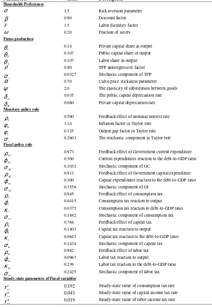
For the set of parameters calibrated to match the moments of data (first and second

moments), we use average ratios for data collected on key macroeconomic variables. The

steady-state values or deterministic equilibrium relationships allow us to assign values to

these parameters. For instance, the static equilibrium derived from the Euler equation

1

18

implies that the discount factor equals the inverse of the gross interest rate 1

r

β

 

=

 

 .

Therefore, we calibrate the parameterβ to match the average T-bill rate

r

. The fraction of saversω is calibrated to 0.20 (20% of households are savers), and the price stickiness

parameter α is calibrated to 0.70 equivalents to average price duration of three quarters.The

risk aversion parameterσ is set to 1.5 according to the literature as well as the labor

substitution parameter

γ

, and the degree of substitution between intermediate goods

ψ

equals 2. For fiscal variables, we use the steady-state values equal to the mean value of each

variable ratio to GDP. These areτ =_ssc 0.192, τ =_ssw 0.019, τ =_ssk 0.043and S_ss =0.37. Table (4) in the appendix provides the calibrated values of parameters in the model.

5.2

Estimation

We estimate the model using seven observable variables on an annual basis: real GDP

( )

Y_t ,

household consumption

( )

C_t , government consumption

( )

G_tC , consumer price index

inflation

( )

π

_t , revenue from consumption tax

( )

τ_tC , revenue from the capital income tax

( )

τ_tk

, and T-bill rate

( )

r_t . The choice of these variables is motivated by the issue of identification of deep parameters in the model and the problem of singularity arising from the choice of

linearly dependent observable variables1. Since the model is log-linearized around its

steady-state, we applied the same transformation to observable variables (the first difference

to the log of each variable), which is equivalent to the closed-form expression of the growth

rate of each variable (figure 2 in appendix).

We perform the estimation using the Bayesian approach, which requires the prior

distribution as well as the support of the distribution of each parameter. As such, we refer to

Herbst and Schorfheide (2016) to choose the prior distribution of the parameters to be

estimated. In literature, the prior of the variances of exogenous shocks follows an inverse

gamma distribution with support

(

0,∞

)

. The autoregressive parameters

(

ρ ρ ρ ρ ρ ρ ρ, _c, _w, _k, _gc, _gi, _r

)

, the discount factor

( )

β

, the Calvo price stickiness parameter

( )

α

, the capital depreciation rates

(

δ δ

_G, _P

)

, the steady-state tax rates

(

τ τ τ_ssc, _ssk, _ssw

)

and the

production function parameters (capital and labor share

θ θ θ

1, 2, 3) have prior distribution Beta

1

19

because they are bounded on

[ ]

0,1 . The risk aversion and labor substitution parameters

follow Gamma distribution. Finally, the parameters relating GDP and debt ratio to fiscal

variables have normal distribution1. For parameters relating GDP and debt to fiscal variables

such as consumption tax, capital income tax, and labor income tax, their priors are set to

normal distribution because of ambiguity underlying the sign of these parameters. We then

perform the identification test on the parameters and find that they are all identified except

the fraction of savers

( )

ω

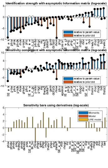
due to the choice of observables available for the estimation.

Therefore it is not estimated. The outcome of the identification test indicates that 99.4% of

the prior support gives a unique saddle-path solution to the model. The sensitivity analysis

shows the importance of parameters on the model in its linear expectation representation and

confirms the identifiability of the parameters (figure 14)2. We conclude that the model does

not feature any identification problems inherent to the structure of the DSGE model. The

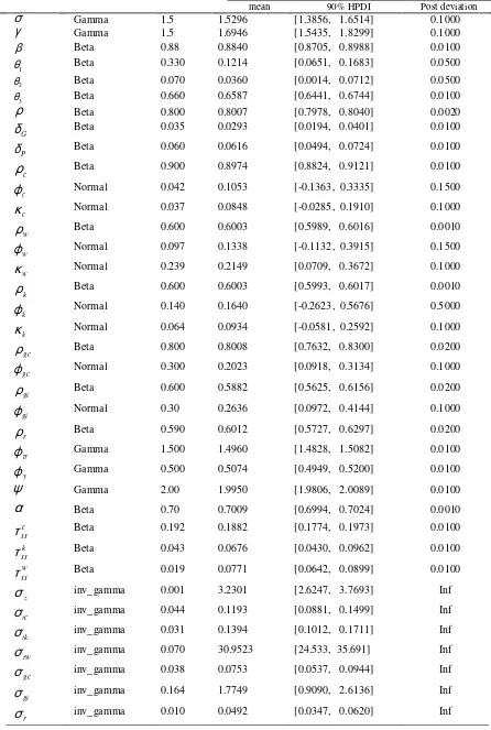
estimation provides the results summarized in table 1. The posterior mean values, the

variances as well as the Highest Probability Density Interval (HPDI) for each parameter are

computed from 10,000 draws from the prior support using Metropolis-Hastings (M-H)

algorithm3.

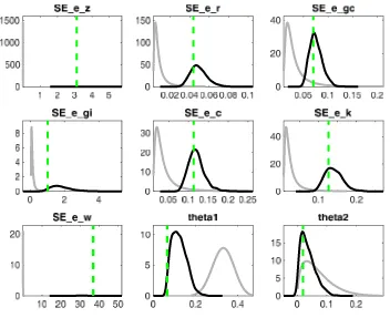
The general picture emerging from the outcomes is that the prior distributions match the

posterior accurately in most cases, suggesting that the information in the data used to

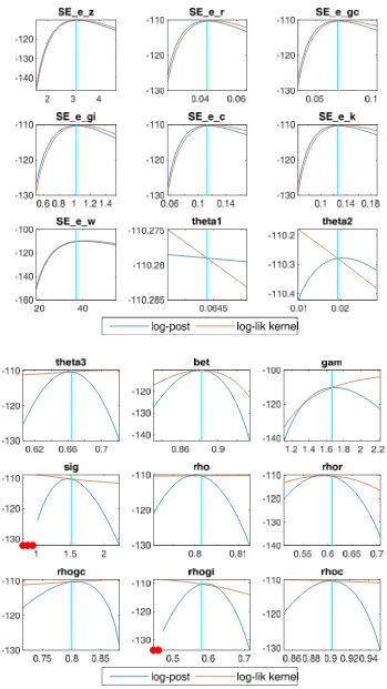
estimate the parameter are consistent with our prior beliefs (figure 16). In addition, figure 15

suggests that the calibrated values of the parameters provide non-explosive solutions to the

model. It also suggests that Blanchard-Kahn conditions are satisfied because the estimated

mode is at the maximum of the posterior likelihood for almost all the parameters4.

The most exciting aspect of these estimates is the steady-state tax rates and the 90% HPDI

derived from the posterior density. It stands out that contrary to the claim that the capital

should not be taxed at steady-state (Chamley (1986), Chari et al. (1991) and others), our

findings reveal a steady-state value of 0.0676 (6.76%) and a range of

[

0.0430, 0.0962

]

within which the fiscal authorities could set the capital income tax. This finding corroborates

the view of Piketty (2015) who argues that capital should be taxed because its return is

always higher than the economic growth throughout history and the gap between the return

1

See Herbst and Schorfheide (2016) for details on Bayesian estimation of DSGE. The choice of prior is guided by the restriction on the domain of some parameters and the uncertainty about the sign

2

See Iskrev (2010b) and Ratto (2011) for details on the Identification test and sensitivity analysis.

3

See Herbst and Schorfheide (2016) for details on the methodology

4

20

to capital and GDP growth is the leading cause of inequality1. Unquestionably, the

steady-state tax on capital income cannot be around zero in a developing economy even though the

capital stock is essential to economic growth and job opportunities. As far as consumption

tax is concerned, our estimates provide a reasonable rate compared to that applicable in

similar economies where the value-added tax (VAT) is 18%. As for the labor income

steady-state tax rate, its value is close to the rate of capital income, and the lower value almost

equal to the posterior mean of the capital income tax.

Further analysis of the estimated parameters of the fiscal rules provides evidence that tax

rates respond positively to explosive domestic debt-to-GDP ratio meaning that fiscal policy

adjusts to any increase of debt-to GDP ratio during the previous period. Additionally, the tax

rates respond positively to the economic situation as the coefficients of the output gap in the

tax rate equations are positive in the three instrument equations. The positive values of the

posterior mean, for the prior normal distribution, illustrate the stabilization role of tax

instruments. However, the 90 % interval encompasses zero for the parameters of output gap

and domestic debt in tax equations. This suggests that fiscal authorities at some time over

the period of the estimation do not consider neither the output gap nor the deviation of

domestic debt from its steady-state to adjust tax rate. This illustrates the time inconsistency

of fiscal policy that could lead to higher than expected domestic debt level2.

Turning to the government spending side, we observe that the estimates of debt-to-GDP

coefficients have the expected sign. Although their prior distributions are normal, their

lower bounds of the 90% HPDI are both positive. This finding supports the idea that

government spending (both consumption and investment) is the main driving force of

domestic debt dynamics.

Equally important is the analysis of the estimated parameters in the Taylor rule, especially

the inflation and output parameters, which reflect the importance of the output gap and

inflation in monetary policy decision by central bank authorities. The prior means for these

two parameters are set to their conventional calibrated values, giving more weight to

inflation and a relatively smaller weight to output, bearing in mind the problem of

indeterminacy. As provided by the estimate, both coefficients are very close to their prior

1

Although our model is not meant to define the optimal taxation for this economy, zero tax on capital income is positively discriminatory to Ricardian households.

2

21

mean values, suggesting that monetary authorities react timely to inflation in a way

consistent with the monetary policy framework.

An important finding which deserves comments is the production function parameters,

especially private capital and labor inputs share. We observe that the estimated values of

these two parameters imply a decreasing return to scale in these two factors. Looking closely

at the 90% interval, we can infer that neither combination of the two parameters yields a

constant or increasing return to scale in labor and private capital meaning that for any two

values from the 90% HPDI of the parameters, the sum is always less than a unit. This feature

is mainly due to the share of private capital, which is lower than the calibrated value.

The estimation provides the magnitude of different shocks in the model as an illustration of

the significance of innovations in the model. The results suggest that the shock to labor

income tax was the most prominent during the period of estimation and contributes to the

fluctuation in all fiscal variables (government spending, debt, and tax rates) as well as output

growth, consumption, and inflation. The productivity shock is another sizeable shock with a

significant contribution to the fluctuation in output growth. The government capital

expenditure shocks have also been sizeable in magnitude. From the historical shock

decomposition, it appears that the fluctuation in the domestic debt stems from the following

shocks: shocks to government capital expenditure, interest rate, labor income tax, and

productivity. The most important contribution to the positive movement of domestic debt

(deviation above its steady-state) arises from positive disturbances in government capital

spending while government consumption spending has no contribution to fluctuation during

the period of estimation.

[image:23.595.79.525.90.753.2]

22

Table 1: Prior and Posterior Distributions of the estimated parameters

Parameters Prior distribution Prior mean Posterior

mean 90% HPDI Post deviation σ Gamma 1.5 1.5296 [1.3856, 1.6514] 0.1000

γ

Gamma 1.5 1.6946 [1.5435, 1.8299] 0.1000

β Beta 0.88 0.8840 [0.8705, 0.8988] 0.0100

1

θ Beta 0.330 0.1214 [0.0651, 0.1683] 0.0500

2

θ Beta 0.070 0.0360 [0.0014, 0.0712] 0.0500

3

θ Beta 0.660 0.6587 [0.6441, 0.6744] 0.0100

ρ

Beta 0.800 0.8007 [0.7978, 0.8040] 0.0020

G

δ

Beta 0.035 0.0293 [0.0194, 0.0401] 0.0100

P

δ Beta 0.060 0.0616 [0.0494, 0.0724] 0.0100

c

ρ

Beta 0.900 0.8974 [0.8824, 0.9121] 0.0100

c

ϕ

Normal 0.042 0.1053 [-0.1363, 0.3335] 0.1500

c

κ

Normal 0.037 0.0848 [-0.0285, 0.1910] 0.1000

w

ρ

Beta 0.600 0.6003 [0.5989, 0.6016] 0.0010

w

ϕ

Normal 0.097 0.1338 [-0.1132, 0.3915] 0.1500

w

κ

Normal 0.239 0.2149 [0.0709, 0.3672] 0.1000

k

ρ

Beta 0.600 0.6003 [0.5993, 0.6017] 0.0010

k

ϕ

Normal 0.140 0.1640 [-0.2623, 0.5676] 0.5000

k

κ

Normal 0.064 0.0934 [-0.0581, 0.2592] 0.1000

gc

ρ Beta 0.800 0.8008 [0.7632, 0.8300] 0.0200

gc

ϕ Normal 0.300 0.2023 [0.0918, 0.3134] 0.1000

gi

ρ Beta 0.600 0.5882 [0.5625, 0.6156] 0.0200

gi

ϕ Normal 0.30 0.2636 [0.0972, 0.4144] 0.1000

r

ρ

Beta 0.590 0.6012 [0.5727, 0.6297] 0.0200

π

ϕ

Gamma 1.500 1.4960 [1.4828, 1.5082] 0.0100

y

ϕ Gamma 0.500 0.5074 [0.4949, 0.5200] 0.0100

ψ

Gamma 2.00 1.9950 [1.9806, 2.0089] 0.0100

α

Beta 0.70 0.7009 [0.6994, 0.7024] 0.0010

c ss

τ Beta 0.192 0.1882 [0.1774, 0.1973] 0.0100

k ss

τ Beta 0.043 0.0676 [0.0430, 0.0962] 0.0100

w ss

τ Beta 0.019 0.0771 [0.0642, 0.0899] 0.0100

z

σ

inv_gamma 0.001 3.2301 [2.6247, 3.7693] Inf

tc

σ

inv_gamma 0.044 0.1193 [0.0881, 0.1499] Inf

tk

σ

inv_gamma 0.031 0.1394 [0.1012, 0.1711] Inf

tw

σ

inv_gamma 0.070 30.9523 [24.533, 35.691] Inf

gc

σ inv_gamma 0.038 0.0753 [0.0537, 0.0944] Inf

gi

σ inv_gamma 0.164 1.7749 [0.9090, 2.6136] Inf

r

23

5.3

The impulse response of endogenous variables to shocks

Based on the parameter values, the time paths of endogenous variables of the model are

simulated following different shocks. We first consider the shocks on fiscal variables

(government expenditure and distortionary tax rates) to assess the impact on fiscal variables

and the domestic debt path. Therefore, the analysis focuses on the effects of fiscal shocks on

the debt path and economic growth and the crowding-out effect on the private sector.

Government spending shocks: The first part of the analysis examines the effect of

expansionary fiscal policy on the dynamic of domestic debt. Figure 3 presents the model

implied impulse response of key variables following a shock to government consumption

spending. As can be seen from the figure, the dynamic of domestic debt has the expected

impulse response to shock on government consumption spending. It appears that the

increase of public consumption spending implies a high growth rate of domestic debt,

contraction of public and private investments. What stands out here is that the increase of

government consumption expenditure implies an increase of domestic debt which crowds

out private investment meaning that any increase in government borrowing leads to a

reduction of access to credit by private sector. The increase of government consumption

spending also leads to the contraction of public investment growth rate. The two effects are

further exemplified by the fact that government consumption shock is not followed by a

convenient tax adjustment policy to provide more revenue. As the impulse response shows,

we observe a little adjustment of different tax rates; yielding a gap between government

revenue and expenditure thus higher domestic debt to finance budget deficit resulting from

the increase in government consumption. Turning to the impact on real variables, it can be

noted that expansionary government spending has a positive impact on output and

households’ consumption as it appears on the impulse response figure 3 . This result was

also reported by Galí et al (2007) in a New Keynesian model with rule-of-thumb

households. According to the literature, the reason for the positive effect of government

spending shock on output and household consumption is the existence of an important

fraction of non-Ricardian households; financially constrained and consume their income

fully in each period as opposed to Ricardian households. Another factor adding to the

positive response of household consumption to government spending shock is the price

stickiness featured in the New-Keynesian model. The estimated value of the Calvo price

stickiness parameter suggests an average price duration of three quarters. This provides

24

to a positive response of consumption following a shock to government spending (Galí et al

2007)1.

In much the same way, a shock to government investment expenditure creates the same

impact on fiscal variables but with different magnitudes as can be seen in figure 42. As it is

noted above, the increase in government capital expenditure leads to a restriction of

government consumption. The same impact on domestic debt occurs as a result of

unchanged tax policy to respond to a higher increase in capital spending. As government

borrowing increases, private sector access to financing shrinks and private investment

growth reduces. As a way of comparison, this type of government spending has a similar

effect on output and household consumption as does the government expenditure.

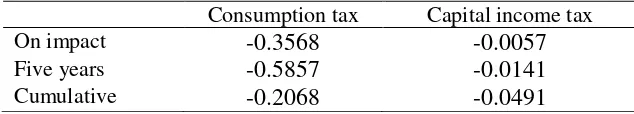
Tax policy shocks: On the revenue side, a shock to consumption tax and capital income tax

leads to a decrease in domestic debt growth. First, figure 5 shows the stabilizing effect of a

shock to consumption tax on the domestic debt through an increase of government revenue;

leading to a reduction of government borrowing. Conversely, households’ consumption

responds negatively especially the consumption of Non-Ricardian households as those