An Improved IS LM Model To Explain Quantitative Easing

Munich Personal RePEc Archive

An Improved IS-LM Model To Explain

Quantitative Easing

Hiermeyer, Martin

26 February 2019

Online at

https://mpra.ub.uni-muenchen.de/92394/

An Improved IS-LM Model To

Explain Quantitative Easing

ByMARTIN HIERMEYER*

The paper combines the IS-LM model with a Tobin-style

analysis of the banking system. As suggested by Krugman,

the resulting model has great predictive power. It can explain

quantitative easing and its effect on the economy, helicopter

money and money creation by banks. Also, it is free of the

normal shortcomings of the IS-LM model.

* German Ministry of Finance, Wilhelmstr. 97, 10117 Berlin (e-mail: [email protected]).

I’m grateful to C.A.E. Goodhart and Peter Howells for many helpful comments.

I. Introduction

The IS-LM model has largely disappeared from research and, to some

extent, also from teaching. This is understandable given the shortcomings

of the model. It is also regrettable given the predictive power of the model.

Krugman (2018) argues that the IS-LM model is in many ways the best

model in all of economics. After all, it was the IS-LM model which

cor-rectly predicted that there would be no surge in inflation when the

Bernanke Fed embarked on quantitative easing and expanded

high-pow-ered money by a factor of almost five. And it was the IS-LM model which

correctly predicted that the 2009 Obama White House fiscal stimulus

would not drive up interest rates. Which other economic model, Krugman

asks, provides such strong, counterintuitive and successful predictions?

Krugman suggests that it takes “IS-LM-with-Tobin” to fully leverage the

IS-LM model’s potential. This paper offers just that. It combines the

IS-LM model with a Tobin (1963)-style analysis of the banking system to

ex-plain quantitative easing, helicopter money and money creation by banks.

2

II. Improved IS-LM Model

The improved IS-LM model is based on three accounting identities and

five plausible assumptions. The accounting identities are given by

equa-tions (1) to (3) while the assumpequa-tions are given by equaequa-tions (4) to (8).

(1) Y  C + I + G

(2) HPM  CHP + ER + RR

(3) RR  rrD, with rr ≥ 0

(4) I = I(lbi), with I’(bli) < 0

(5) HPM = HPM(ffr), with HPM’(ffr) < 0

(6) CHP = CHP(bli), with CHP’(bli) < 0

(7) ER = ER(bli), with ER’(bli) < 0

(8) D = D(Y), with D’(Y) > 0

The variables are:

Y: Output ER: Excess reserves

C: Consumption spending RR: Required reserves

I: Investment spending rr: Reserve ratio

G: Government spending D: Demand deposits

HPM: High-powered money bli: Bank loan interest rate

CHP: Currency held by the public ffr: Federal funds rate

Equation (1) is the national income identity for a closed economy.

Equa-tion (2) defines the components of high-powered money. EquaEqua-tion (3)

de-fines the reserve ratio.

Equation (4) assumes that investment spending decreases with the bank

loan interest rate. This is plausible as a higher bank loan interest rate means

that some investment projects are no longer profitable.

Equation (5) assumes that demand for high-powered money decreases

3

interest rate which banks pay when they borrow high-powered money from

the Fed.

Equation (6) assumes that the amount of currency held by the public

de-creases with the bank loan interest rate. This is plausible as a higher bank

loan interest rate generally comes with a higher savings accounts interest

rate which makes it more attractive for the public (i.e. households and

firms) to reduce currency balances by paying some currency into savings

accounts.

Equation (7) assumes that the amount of excess reserves held by banks

decrease with the bank loan interest rate. This is plausible as the bank loan

interest rate reflects banks’ opportunity cost of holding excess reserves

in-stead of making loans.

Equation (8) assumes that demand deposits increase with output. This is

plausible as additional output implies additional transactions. Additional

transactions imply additional demand deposits, as payment with check,

di-rect debit or bank wire transfer is generally the main method of payment.

The improved IS-LM model consists of an improved IS curve and an

improved LM curve.

The improved IS curve is obtained by combining equations (1) and (4).

(I-IS) Y = C + I(bli) + G, with I’(bli) < 0

Combining equations (2), (3) and (5) to (8) yields the improved LM curve.

(I-LM) HPM(ffr) = CHP(bli) + ER(bli) + rrD(Y),

with HPM’(ffr) < 0, CHP’(bli) < 0, ER’(bli) < 0 and D’(Y) > 0

III. Improved IS-LM Model Versus IS-LM Model

The improved IS-LM model is similar to the IS-LM model. Developed

by Hicks (1937) and Hansen (1953), the IS-LM model consists of an IS

curve and an LM curve.

4

(LM) M = L(i, Y), with L’(i) < 0 and L’(Y) > 0

The variables, if not already defined, are:

i: Interest rate L: Liquidity demand

M: Money supply

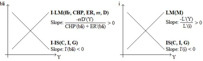
Figure 1 compares the improved IS-LM model to the IS-LM model. As can

be seen, the improved IS-LM operates in output-bank loan interest rate

space rather than in output-interest rate space. Also, the improved LM

curve has four endogenous variables more than the LM curve. The

im-proved IS curve and the IS curve have the same slope if I’(i) = I’(bli) holds.

The improved LM curve and the LM curve have the same slope if L’(Y) =

rrD’(Y) and L’(i) = CHP’(bli) + ER’(bli) holds.

FIGURE 1.IMPROVED IS-LMMODEL VERSUS IS-LMMODEL.

IV. How The Improved IS-LM Model Works

To understand how the improved IS-LM model works, consider a

mon-etary expansion in the model. For HPM’(ffr)=-4, I’(bli)=-20, CHP’(bli)=

-1, ER’(bli)=-1, rr=0.1 and D’(Y)=1, a 1 percentage point cut in the federal funds rate leads to a $20 increase in output, as shown by equation (9).

(9) 𝑑𝑌

𝑑𝑓𝑓𝑟 =

𝐻𝑃𝑀′_{(𝑓𝑓𝑟) 𝐼}′_{(𝑏𝑙𝑖)}

𝐶𝐻𝑃′_{(𝑏𝑙𝑖) + 𝐸𝑅}′_{(𝑏𝑙𝑖) + 𝑟𝑟𝐷}′_{(𝑌) 𝐼}′_{(𝑏𝑙𝑖)} =

80 −4 = -20

Figure 2 shows this graphically, assuming arbitrary initial values for the

federal funds rate, output and the bank loan interest rate. As can be seen,

the 1 percentage point reduction in the federal funds rate from 2% to 1%

5

FIGURE 2.REDUCTION IN THE FEDERAL FUNDS RATE IN THE IMPROVED IS-LMMODEL.

Table 1 compares point C – the initial equilibrium – to point A – the new

equilibrium – and shows how the variables in equations (I-IS) and (I-LM)

change. Several things can be seen.

TABLE 1—CHANGE IN THE INVOLVED VARIABLES:POINT CVERSUS POINT AOF FIGURE 2 (1) Change in the federal funds rate (ffr) -1 percentage point (2) Change in high-powered money (HPM)

+$4 (3) Change in the bank loan interest rate (bli) -1 percentage point (4) Change in currency held by the public (CHP) +$1 (5) Change in excess reserves (ER) +$1 (6) Change in the bank loan supply +$20 (7) Change in demand deposits (D) +$20 (8) Change in required reserves (RR) +$2 (9) Change in bank loan demand +$20 (10) Change in investment (I) +$20 (11) Change in output (Y) +$20

Line 2: The 1 percentage point cut in the federal funds rate comes with a

$4 increase in high-powered money as the Fed’s New York traders lend an

additional $4 of high-powered money to banks to implement the Federal

Open Market Committee’s decision regarding the federal funds rate. Line 3: The reduction in the federal funds rate comes with a 1 percentage

point reduction in the bank loan interest rate.

Lines 4 and 5: The lower bank loan interest rate makes it more attractive

for the public to hoard currency by withdrawing currency from savings

ac-counts and makes it more attractive for banks to hoard excess reserves. Of

the $4 increase in high-powered money, $1 is absorbed into currency held

by the public and $1 into excess reserves. This leaves $2 of high-powered

money to hit the real economy.

Lines 6, 7 and 8: Those $2 of high-powered money that hit the real

6

making loans. When banks make loans, they credit the demand deposit

ac-counts of the firms with a demand deposit of the size of the loan so that the

firms can use the money. Thus, both bank loan supply and demand deposits

are up by $20. Since the reserve ratio is assumed to be 0.1, required reserves

are up by $2.

Lines 9, 10 and 11: Like the bank loan supply, bank loan demand is up

by $20 as the lower bank loan interest rate makes firms borrow and invest

$20 more. When the firms spend the additionally borrowed $20, output

in-creases by $20 as prices are assumed to be fixed in the short run.

A. Monetary Policy Is Partly Self-Defeating

Figure 2 shows that monetary policy is partly self-defeating. The increase

in output would be greater if the bank loan interest rate would not decline

so that none of the additional high-powered money is absorbed into idle

currency held by the public and excess reserves. Such a happy “state of affairs” is the case at point B of Figure 2. However, as Table 2 shows, point

B is no equilibrium as bank loan supply (line 6) exceeds bank loan demand

(line 9) by $40 there.

TABLE 2—CHANGE IN THE INVOLVED VARIABLES:POINT BVERSUS POINT AOF FIGURE 2 (1) Change in the federal funds rate (ffr) -1 percentage point (2) Change in high-powered money (HPM) +$4 (3) Change in the bank loan interest rate (bli) Unchanged (4) Change in currency held by the public (CHP) Unchanged (5) Change in excess reserves (ER) Unchanged (6) Change in the bank loan supply +$40 (7) Change in demand deposits (D) +$40 (8) Change in required reserves (RR) +$4 (9) Change in bank loan demand Unchanged

B. Bonds Instead Of Bank Loans

The aforesaid assumes that banks create demand deposits by making

loans and crediting the proceeds to the borrower’s demand deposits

ac-count. However, banks might just as well create demand deposits by

pur-chasing bonds and crediting the proceeds to the bond issuer’s demand

7

In this case, the following replacements are necessary in Tables 1 and 2:

“bond market interest rate” instead of “bank loan interest rate” in line (3),

“bond demand” instead of “bank loan supply” in line (6), and “bond

sup-ply” instead of “bank loan demand” in line (9).

It is also conceivable that banks create additional demand deposits partly

through loans and partly through bonds. In this case, the appropriate terms

are “credit market interest rate”, “credit supply” and “credit demand”.

V. Improved IS-LM Model And Quantitative Easing

Equation (9) shows that monetary policy becomes ineffective under

cer-tain conditions. Those conditions are summarized in Table 3.

TABLE 3—CONDITIONS WHICH RENDER MONETARY POLICY INEFFECTIVE

Condition Effect on curve Economic intuition

ER’(bli)→∞ Horizontal improved LM curve Banks are unwilling to make loans and rather hoard excess reserves

I’(bli)=0 Vertical improved IS curve Firms are unwilling to borrow

HPM’(ffr)=0 Horizontal improved LM curve Banks are unwilling to borrow high-powered money from the Fed

CHP’(bli)→∞ Horizontal improved LM curve The public hoards as much currency as possible

D’(Y)→∞ Horizontal improved LM curve Firms are unwilling to spend borrowed money rr→∞ Horizontal improved LM curve The Fed sets an extremely high reserve ratio

If one of those conditions holds, or nearly holds, the effectiveness of

monetary policy is hampered, and the Fed may undershoot its inflation

tar-get. In response, the Fed may drive the federal funds rate down to zero.

Once there, the Fed may wish to resort to quantitative easing if inflation is

still too low.

In quantitative easing, the Fed purchases financial assets from banks with

high-powered money. Despite the additional high-powered money, the

fed-eral funds rate does not go any lower as it has already reached its zero lower

bound.

The improved IS-LM model can show quantitative easing. For

HPM’(ffr)=0, high-powered money becomes exogenous and the Fed can increase it directly. Equation (10) shows the effect of such a direct increase

8

(10) _{𝑑𝐻𝑃𝑀}𝑑𝑌 = _{𝐶𝐻𝑃′} 𝐼′(𝑏𝑙𝑖)

(𝑏𝑙𝑖) + 𝐸𝑅′_{(𝑏𝑙𝑖) + 𝑟𝑟𝐷}′_{(𝑌) 𝐼}′_{(𝑏𝑙𝑖)}

Equation (10) is equal to equation (7) with the only exception that the term

HPM’(ffr) no longer appears. Given the similarity of both equations, it follows that if the efficiency of conventional monetary policy is restricted

by an unfavorable parameter other than HPM’(ffr), quantitative easing is

suffering, too.

If quantitative easing is more effective than conventional monetary

pol-icy, then only because of scale. In quantitative easing, the Fed can increase

high-powered money quite drastically. For example, following the

finan-cial crisis, the Fed increased high-powered money by a factor of almost

five.

A. LM Channel of Quantitative Easing

If the improved LM curve is minimally upward sloping rather than flat

and if the improved IS curve is not vertical, sheer mass may make

quanti-tative easing somewhat effective. A small portion of the flood of

high-pow-ered money may trickle into the real economy, leading to some increase in

bank loans, demand deposits, required reserves and output. The remainder

of the additional high-powered money ends up idly as currency held by the

public and/or excess reserves.

B. IS Channel of Quantitative Easing

There is also the possibility that the flood of high-powered money shifts

the improved IS curve to the right. This is not modelled here, yet it is

con-ceivable. In this case, output will increase if the improved LM curve is not

vertical which most likely it isn’t as otherwise monetary policy would be

highly effective and there would be no need to resort to quantitative easing

in the first place.

The ratio of the increase in high-powered money to the prompted shift in

the improved IS curve will probably be large, so that most of the additional

9

excess reserves. Again, a small portion may however trickle into the real

economy as some firms are willing to borrow and spend additional money

because of quantitative easing and its effect on credit conditions.

Then Fed chairman Ben Bernanke emphasized the “IS channel” in 2009

when the Fed embarked on quantitative easing. Bernanke went so far as to

make a distinction between “pure” quantitative easing as employed by the Bank of Japan from 2001 to 2006 and the Fed’s approach (Bernanke 2009).

While he admitted that both approaches involve an expansion of the

cen-tral bank’s balance sheet, he argued that in pure quantitative easing, the

focus of policy is the quantity of bank reserves, which are liabilities of the

central bank; at the same time, the composition of loans and securities on

the asset side of the central bank’s balance sheet is only incidental.

In contrast, according to Bernanke, the Fed’s credit easing approach

fo-cused on the mix of loans and securities that it holds and on how this

com-position of assets affects credit conditions for households and businesses.

Bernanke even tried to call the Fed’s new policies “credit easing” to distin-guish it from pure quantitative easing. However, as Blinder (2010) notes,

the label did not stick.

C. Predictive Power Of The Improved IS-LM Model

Irrespective of whether quantitative easing works through the IS channel

or the LM channel, the improved IS-LM model suggests that even very

large increases in high-powered money affect output (and/or prices if the

latter are flexible) only modestly if quantitative easing is employed in a

situation where unfavorable parameters hamper conventional monetary

policy. Instead, only currency held by the public and/or excess reserves go

through the roof.

This is a good prediction. US quantitative easing increased output and

prices by only 26% between January 2008 and December 2015. At the

same time, it increased excess reserves by 140,000% (Federal Reserve

10

but apparently also a counterintuitive one as there were many people who

predicted that quantitative easing would lead to high inflation.

If it is a flat improved LM curve that gives rise to quantitative easing, the

improved IS-LM model suggests furthermore that fiscal stimulus does not

drive up interest rates when employed alongside quantitative easing. As

Krugman (2018) notes, this is another counterintuitive IS-LM prediction

which came true recently.

VI. Improved IS-LM Model And Helicopter Money

From the aforesaid it follows that quantitative easing does not work if (a)

the improved LM curve is horizontal and if (b) the improved IS curve does

not react to quantitative easing.

In such a case, the Fed may want to attack the IS curve directly. This is

called helicopter money.

In helicopter money, the Fed uses newly created high-powered money to

acquire demand deposits at banks. The Fed then gifts the demand deposits

to households or, alternatively, to the government. While it is not clear

whether households will spend the money so received, it seems certain that

the government would agree to do so if this is necessary to combat

defla-tion. If helicopter money is distributed to the government, the process is

also known as government debt monetization.

This mechanism is very powerful as both the improved LM curve and

the improved IS curve shift to the right here. In fact, this is the very

mech-anism through which all past hyperinflations came about.

VII. Improved IS-LM Model And Money Creation By Banks

As McLeay et al. (2014) note: In the modern economy, most money takes

the form of demand deposits and is created endogenously by banks. The

improved IS-LM model reflects that. This is a major step forward when

compared to the IS-LM model which assumes that all money is created by

11

A. Tobin’s (1963) Analysis Of The Banking System

The improved IS-LM model also drives home a point made by Tobin

(1963), namely that banks do not possess a “widow’s cruse”. There are

limits to the banking systems’ capability to create money as “Marshall’s

scissors of supply and demand” apply also to the output of the banking

industry (i.e. to bank loans and demand deposits). If demand deposits are

excessive relative to public preferences, Tobin argued, they will tend to

decline, and banks cannot do anything about it.

The improved LM and IS curves reflect Marshall’s scissors of supply and

demand. Banks can create additional demand deposits only subject to

pub-lic preferences. If there is no demand for loans, that is, if the improved IS

curve is vertical, banks cannot create additional demand deposits at all.

For a non-vertical improved IS curve, banks can create additional

de-mand deposits (a) because they themselves choose to do so by exogenously

decreasing excess reserves, or (b) because the Fed, households, firms or the

government curve induce them to do so.

B. Fed- And Non-Fed-Induced Money Creation By Banks

How the Fed can induce banks to create additional demand deposits was

described in chapter IV. There, a 1 percentage point reduction in the federal

funds rate made banks create $20 in additional demand deposits. The

pro-cess is governed by equation (11).

(11) 𝑑𝐷

𝑑𝑓𝑓𝑟 =

𝐻𝑃𝑀′_{(𝑓𝑓𝑟) 𝐼}′_{(𝑏𝑙𝑖) 𝐷}′_(𝑌)

𝐶𝐻𝑃′_{(𝑏𝑙𝑖) + 𝐸𝑅}′_{(𝑏𝑙𝑖) + 𝑟𝑟𝐷}′_{(𝑌) 𝐼}′_{(𝑏𝑙𝑖)} =

80 −4 = -20

Next to the Fed, households, firms and the government can induce banks

to create additional demand deposits. Equation (12) shows how a $1

increase in, here, consumption spending makes banks create $0.5 in

additional demand deposits for the parameters from chapter IV.

(12) 𝑑𝐷

𝑑𝐶 =

𝐶𝐻𝑃′_{(𝑏𝑙𝑖) 𝐷}′_{(𝑌) + 𝐸𝑅}′_{(𝑏𝑙𝑖) 𝐷}′_(𝑌)

𝐶𝐻𝑃′_{(𝑏𝑙𝑖) + 𝐸𝑅}′_{(𝑏𝑙𝑖) + 𝑟𝑟𝐷}′_{(𝑌) 𝐼}′_{(𝑏𝑙𝑖)} =

12

The same expression holds for an increase in investment or government

spending. Equation (12) drives home the point of Goodhart (2017) that

banking is a service industry which sets the terms and conditions whereby

the private and government sector can create additional money for itself.

VIII. Eliminated Shortcomings Of The IS-LM Model

As a welcome side-effect, the improved IS-LM model eliminates all the

shortcomings of the standard IS-LM model.

A. Unlike The IS-LM Model, The Improved IS-LM Model Does Not

Assume That The Fed Targets Money

The IS-LM model assumes wrongly that the Fed targets money, and more

specifically the money supply M. In principle, the Fed might do so by

set-ting a target path for M or by explicitly changing M from time to time, for

example after a Federal Open Market Committee (FOMC) meeting.

This is, however, not how the Fed conducts monetary policy today.

Ra-ther, the Fed targets the federal funds rate: The FOMC from time to time

decides upon a change in the federal funds rate and the Fed’s New York

traders continuously adjust a measure of the money supply (high-powered

money) as necessary to keep the federal funds rate as close as possible to

the FOMC’s target. The improved IS-LM model fully reflects that.

B. Unlike The IS-LM Model, The Improved IS-LM Model Is Clear

About Its Money Measures

The IS-LM model is unclear about the LM curve’s money measures M

and L. Very few authors are willing to take a stance whether M and L

re-flect high-powered money, M1 money or some entirely different money

measure.

In contrast, the improved LM curve is clear about its money measures

which are: High-powered money, currency held by the public, excess

13

High-powered money gives the Fed’s leverage over the economy: Banks

need it because the public demands currency and/or because the Fed

de-mands required reserves; at the same time, only the Fed can create it.

Demand deposits underlie transactions which in turn underlie additional

output. Equation (4) assumed that all transactions are settled cashless

through demand deposits as output is not related to currency held by the

public. For added realism, one could also allow for cash transactions. In

this case, in equation (4), the demand for currency held by the public would

depend not only negatively on the bank loan interest rate but also positively

on output.

C. Unlike The IS-LM Model, The Improved IS-LM Model Is Clear

About Its Interest Rate

The IS-LM model is unclear about its interest rate i. Very few authors

are willing to take a stance whether i reflects the federal funds rate, the

bank loan interest rate or some entirely different interest rate.

In contrast, the improved IS-LM model is clear about its interest rates

which are the federal funds rate and the bank loan interest rate.

The federal funds rate is the Fed’s policy rate and the Fed manipulates

high-powered money as necessary to achieve its target for the federal funds

rate. The bank loan interest rate matches demand and supply for bank loans.

As discussed in section IV B, the interest rate can be generalized to a bond

market interest rate or a credit market interest rate.

IX. Conclusion

The improved IS-LM model puts flesh on the bones of the IS-LM model.

While it maintains the IS-LM model’s basic structure, it is more precise

14

TABLE 4—THE IMPROVED IS-LMMODEL PUTS FLESH ON THE BONES OF THE IS-LMMODEL

Variables of the IS-LM Model Variables of the Improved IS-LM Model

Output (Y) Output (Y) Interest rate (i) Bank loan interest rate (bli)

Federal funds rate (ffr)

Consumption spending (C) Consumption spending (C) Investment spending (I) Investment spending (I) Government spending (G) Government spending (G)

Money (M) High-powered money (HPM) Liquidity (L) Currency held by the public (CHP)

Excess reserves (ER) Demand deposits (D)

This paper is not the first attempt to improve the IS-LM model in general

and the LM curve in particular.

Bernanke and Blinder (1988) suggest a modified LM curve which

in-cludes bank reserves to analyze the relative merits of bank assets and bank

liabilities as indicators and targets of monetary policy. Since Bernanke and

Blinder were not interested in quantitative easing or helicopter money, their

LM curve does however not include high-powered money as an entity

sep-arate from reserves. Nor does it include excess reserves or the federal funds

rate to distinguish quantitative easing from conventional monetary policy.

More recently, Mierau and Mink (2018) suggest a modified LM curve

which includes bank equity to analyze the role of capital requirements in

the transmission of monetary policy. Like Bernanke and Blinder, Mierau

and Mink do not attempt to explain quantitative easing and helicopter

money and so their model doesn’t include high-powered money or excess reserves.

Many other authors have discarded the LM curve all together. Following

Clarida et al. (1999), interest rate rules have displaced the LM curve in

most research.

In teaching, the LM curve has held its ground better. Mankiw (2006)

gives detailed reasons why, for teaching, he continuous to prefer the LM

curve to an interest rate rule. Next to Mankiw (2016), other textbook

au-thors who uphold the IS-LM model include Abel, Bernanke and Croushore

2017, Blanchard 2017, Dwivedi 2015, Froyen 2013 or Heijdra 2017.

15

Allsopp and Vines (2000), Taylor (2000), Walsh (2002), Carlin and

Soskice (2005) or Bofinger et al. (2006) have suggested simple models that

replace the LM curve with an interest rate rule.

The aforesaid sketches the competition and the environment which the

improved IS-LM model faces. Naturally, for the improved IS-LM model

to succeed, it must be superior to the other models, at least for some

appli-cations. Table 5 provides a comparison on which the improved IS-LM

model might stake its claim.

TABLE 5—IMPROVED IS-LMMODEL VERSUS OTHER MODELS

Improved IS-LM Model

Standard IS-LM Model

Interest Rate Rule

Bernanke/ Blinder Mierau/Mink Assumes that the Fed targets the federal

funds rate in conventional monetary ✓  ✓ 

policy?

Shows how the Fed targets the federal

funds rate by manipulating high- ✓    powered money?

Is clear about its money measure(s) (if

any are included in the model) and its ✓  ✓ ✓

interest rate(s)?

Recognizes that most of today’s broad

broad money is created by banks and not ✓   ✓

by the Fed?

Can explain quantitative easing and

helicopter money (including government ✓   

16 REFERENCES

Abel, Andrew B., Ben S. Bernanke, and Dean Croushore. 2017. “Macroe-conomics”, 9th ed. Boston: Pearson Education, Inc.

Allsopp, Christopher and David Vines. 2000. “The Assessment:

Macroe-conomic Policy”. Oxford Review of Economic Policy 16(4): 1-32.

Blanchard, Olivier. 2017. “Macroeconomics”, 7th ed. Upper Saddle River, New Jersey: Pearson Education, Inc.

Bernanke, Ben and Alan Blinder. 1988. “Credit, money and aggregate

de-mand.” American Economic Review, 78(2):435–39.

Bernanke, Ben S. 2009. “The Crisis and the Policy Response”, At the Stamp Lecture, London School of Economics, London, England.

Blinder, Alan S. 2010. “Quantitative Easing: Entrance and Exit Strategies”, Federal Reserve Bank of St. Louis Review, November/December 2010,

92(6): 465-79.

Bofinger, Peter, Eric Mayer and Timo Wollmershäuser. 2006. “The BMW

Model: A New Framework for Teaching Monetary Economics. The

Jour-nal of Economic Education, vol. 37(1).

Carlin Wendy & Soskice David, 2005. “The 3-Equation New Keynesian

Model – A Graphical Exposition”. The B.E. Journal of Macroeconomics,

vol. 5(1), 1-38.

Clarida, Richard, Jordi Gali, and Mark Gertler. 1999. “The Science of

Monetary Policy: A New Keynesian Perspective.” Journal of Economic

Literature, vol. 37 (4): 1661-1707.

Dwivedi, D.N.. 2015. “Macroeconomics – Theory and Policy”, 4th ed.

New York: McGraw-Hill Irwin.

Federal Reserve. 2018. “St. Louis Adjusted Monetary Base”, “Excess Re-serves of Depository Institutions” and “Gross Domestic Product”,

re-trieved from FRED, Federal Reserve Bank of St. Louis.

Froyen, Richard T.. 2013. “Macroeconomics”, 10th ed. Upper Saddle River, New Jersey: Pearson Education, Inc.

Goodhart, C.A.E.. 2017. “The Determination of the Money Supply:

17

Hansen, Alvin H.. 1953. “A Guide to Keynes”. New York: McGraw Hill.

Heijdra, Ben J.. 2017. “Foundations of Modern Macroeconomics”, 3rd _ed.

Oxford University Press.

Hicks, John R. 1937. “Mr. Keynes and the 'Classics': A Suggested

Inter-pretation”. In Econometrica 5 (2). 147-159.

Krugman, Paul. 2018. “What Do We Actually Know About the Economy?” Opinion. New York Times.

https://www.nytimes.com/2018/09/16/opin-ion/what-do-we-actually-know-about-the-economy-wonkish.html

Mankiw, N. Gregory. 2006. “The IS-LM Model”. http://gregmankiw.blog-spot.com/2006/05/is-lm-model.html

Mankiw, N. Gregory. 2016. “Macroeconomics”, 9th ed. New York: Worth Publishers.

McLeay, Michael, Radia, Amar, and Ryland Thomas. 2014. “Money crea-tion in the modern economy.” Bank of England Quarterly Bulletin.

Mierau, Jochen O. and Mark Mink. 2018. “A Descriptive Model of

Bank-ing and Aggregate Demand”, De Economist 166. 207–237.

Romer, David, H.. 2000. “Keynesian Macroeconomics without the LM Curve.” In Journal of Economic Perspectives, 14(2): 149-169.

Taylor, John B. 2000. “Teaching Modern Macroeconomics at the

Princi-ples Level”. American Economic Review Papers and Proceedings 90(2),

90-94.

Tobin, James. 1963. “Commercial banks as creators of money”. Cowles

Foundation Discussion Papers 159, Cowles Foundation for Research in

Economics, Yale University.