Munich Personal RePEc Archive
Exact Likelihood Estimation and
Probabilistic Forecasting in Higher-order
INAR(p) Models
Lu, Yang
University of Paris 13
1 January 2018
Online at
https://mpra.ub.uni-muenchen.de/83682/
Exact Likelihood Estimation and Probabilistic Forecasting
in Higher-order INAR(
p
) Models
Yang Lu
∗January 5, 2018
Abstract: The computation of the likelihood function and the term structure of probabilistic
forecasts in higher-order INAR(p) models are qualified numerically intractable and the literature has considered various approximations. Using the notion of compound autoregressive process,
we propose anexact and fast algorithm for both quantities. We find that existing approximation schemes induce significant errors for forecasting.
Keywords: compound autoregressive process, probabilistic forecast of counts, matrix
arith-metic.
MSC code: 62-15, JEL code: C32
1
Introduction
INteger-valued AutoRegressive process (INAR) has recently received wider attention in the
liter-ature. The benchmark model, introduced by McKenzie (1985), Al-Osh and Alzaid (1987) in the
first-order case (called INAR(1)) and Du and Li (1991) in the higher-order case (called INAR(p)), postulates that:
Xt= p X i=1
αi◦Xt−i+ǫt, ∀t, (1)
where the binomial thinning operators αi ◦Xt−i, with i and t varying, are mutually
Binom(Xt−i, α), whereas the innovation process(ǫt)is i.i.d. and PoissonP(λ)distributed.
Since these seminal works, many extensions of the above model have been proposed. However,
besides the basic INAR(1), the computation of the likelihood function and/or that of the
multi-step-ahead conditional probability mass function (p.m.f.) in higher-order models are documented
to be intractable and various approximation methods are proposed [see e.g. Pedeli et al. (2015) for
estimation and Jung and Tremayne (2006); McCabe et al. (2011) for forecasting]. These methods
can induce significant approximation errors, and some are still computationally intensive. This
paper solves these two difficulties using the compound autoregressive (CaR) property of the
INAR(p) model. Relying on simple, matrix algebra, we obtain a fast and unified algorithm for the two aforementioned quantities, without making any approximation error. Moreover, the
methodology is applicable to a very wide range of INAR(p)models beyond the benchmark case. The paper is organized as follows. Section 2 reviews a natural link between the probability
generating function (p.g.f.) and the probability mass function (p.m.f.) for a count distribution.
Section 3 computes the Taylor’s expansion of the one-step-ahead conditional p.g.f. and deduce
the corresponding p.m.f., which allows for likelihood-based estimation. Section 4 deals with
forecasting and adapts the approach to deduce multiple-step-ahead p.m.f.’s. Section 5 concludes.
2
Link between the p.g.f. and p.m.f. of a count
distribu-tion
LetX be a count variable with known p.g.f.:
φ(u) =E[uX] =
∞
X n=0
unp(n),
where argument u ≥ 0. The aim is to compute the p.m.f. p(n), for any n ∈ N. While the
analogous problem for continuous distributions usually involve approximation methods [see e.g.
distribution. Indeed, the Taylor-expansion (atu= 0) of the p.g.f. is:
φ(u) =
∞
X n=0
φ(n)(0)
n! u
n
.
thus by identification we have:
p(n) = φ
(n)(0)
n! . (2)
Hence the p.m.f. can be computedexactly, so long as the Taylor’s expansion ofφis tractable. Example 1. For instance, if X follows Poisson P(λ) distribution, then we have: φ(u) =
eλ(u−1)=
e−λP∞
n=0 un
n!. Thus we recover the p.m.f. p(n) =e
−λ λn
n!.
3
Likelihood-based estimation
Let us now explain how to adapt this idea to the context of count process. In order to conduct
maximum likelihood (ML) estimation, we have to derivep(·|Xt−1), i.e. the conditional p.m.f. of
Xt given the past Xt−1. This latter distribution is the convolution ofp binomial distributions
αi◦Xt−i,i= 1, ..., p, as well as the Poisson distribution ofǫt. Thus we have [see e.g. Drost et al.
(2009)]:
p(Xt|Xt−1) =
X
n1+n2+···+np+np+1=Xt
p Y j=1
P[αi◦Xt−i=ni]
P[ǫt=np+1]. (3)
The RHS involves a p−dimensional summation, that is a complexity of O(Xtp). This explains
why ML estimation has not yet been considered for INAR(p) models1
withp≥3. While moment based estimators are generically consistent [see e.g. Al-Osh and Alzaid (1987)], they can suffer
from significant efficiency loss [see e.g. Bu et al. (2008)]. Recently, Pedeli et al. (2015) propose a
saddle-point approximation ofp(·|Xt−1). Its drawbacks is, first, the approximatedp(n|Xt−1)does
not sum up to one whennvaries acrossN. Second, the saddle-point itself has to be approximated
numerically, resulting in further computational complexity and approximation error. Pedeli et al.
(2015) show that for certain parameter values, the relative error of the likelihood function can
be as large as2−5percent. As a consequence, their approximate ML estimator is not consistent
1
and simulation results (see their Table 1) show that in finite sample, the bias can be significantly
larger than that of the exact ML estimator.
Our solution consists in first computing the n−th Taylor’s expansion (at zero) of the corre-sponding conditional p.g.f.:
E[uXt|X
t−1] = exp
h p X i=1
Xt−ilog(αiu+ 1−αi) +λ(u−1)
i
(4)
= exph−λ+
p X i=1
Xt−ilog(1−αi) +λu+
p X i=1
Xt−ilog(1 +
αi
1−αi
u)i
= exph−λ+
p X i=1
Xt−ilog(1−αi)
i
exphλu+
p X i=1
Xt−i
n X j=1
(−1)j−1
j ( αi
1−αi
)juj+O(un+1)i
= exph−λ+
p X i=1
Xt−ilog(1−αi)
i
exph
n X j=1
Ajuj i
+O(un+1)
= exph−λ+
p X i=1
Xt−ilog(1−αi)
iXn
k=0
1
k!
hXn
j=1
Aiuj ik
+O(un+1), (5)
where for the computation of the likelihood function, we typically taken=Xt, and coefficients
Ai are given by:
A1=λ+ p X i=1
Xt−i
αi
1−αi
,
Aj =
(−1)j−1
j
p X i=1
Xt−i(
αi
1−αi
)j, ∀j= 2, ..., n.
Thus by equation (2), the probabilityp(n|Xt−1)is the coefficient in front of the termu
n in the
expansion (5). Hence it suffices to compute recursively then+ 1first terms of the polynomial
hPn i=1Aiui
ik
for eachk. While such an expansion can be obtained using a symbolic calculation package such as Mathematica, the following proposition provides a matrix-based algorithm that
is simple for statistical packages2 .
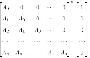
Proposition 1. The n+ 1first coefficients of polynomial hA0+Pnj=1Aiui ik
, wherek= 0, ...n
2
are given by the column vector:
A0 0 0 · · · 0
A1 A0 0 · · · 0
A2 A1 A0 · · · 0
· · · ·
An An−1 · · · A1 A0
k 1 0 0 · · · 0 . (6)
The proof is obvious and omitted. In our case we haveA0= 0, thus the square matrix above
is triangular inferior.3
We can also remark that on the contrary to formula (3), which becomes
cumbersome so long aspis mildly large, in our approach, the computational cost is essentially independent of the value ofp.
To illustrate the computational gain, we implement the likelihood function using both our
new method and the direct method based on (3). We consider an INAR(2) model4
as well
as an INAR(5) model5
. For both models, we simulate trajectories with different sample sizes
T = 100,500and2500, respectively and compute the likelihood function using the two methods.6 The following table compares the execution time in R of the two methods on a standard laptop.
We do not report the likelihood values obtained from these two methods as they coincide with
each other.
Model INAR(2) INAR(5)
Sample size T = 100 T = 500 T = 100 T = 500
Our method 0.002 s 0.010 s 0.002 s 0.009 s
[image:6.595.219.377.131.233.2]Direct method 0.001 s 0.007 s 0.060 s 0.192 s
Table 1: Execution time of the two methods. The time unit is second.
We can see that when the orderpof the INAR model is small (i.e. p= 2), both methods are
3
This square matrix is known as the Toeplitz matrix in the literature.
4
The parameters of the model are fixed as:
α1= 0.8, α2= 0.1, λ= 0.5, (7)
with initial valuesX1=X2= 1.
5
The parameters of this model are fixed as:
α1= 0.3, α2= 0.2, α3= 0.1, α4= 0.05, α5= 0.01, λ= 1, (8)
with initial valuesX1=· · ·=X5= 1.
6
fast. This is understandable, since for this model, the computation of the conditional p.g.f. has a
complexity ofO(Xt3)for both models. Whenpincreases to 5, our method becomes dominant, as
its computational cost remains nearly unchanged whereas the direct method is 25 times slower.
To summarize, the simplicity of our approach is mainly due to equation (4), which says
that the one-step-ahead conditional p.g.f. is an exponential linear function of past observations.
Such processes(Xt)are called (p−th order) compound autoregressive (CaR(p)) processes in the
general time series literature [see Darolles et al. (2006)]. Their analysis is generically simple
using the conditional p.g.f.7
. Here since we have a count distribution, the p.m.f. is also easily
computable.
4
Multi-step forecasting
While the conditional meanE[Xt+h|Xt−1]is simple to obtain for the INAR(p) model [see e.g. Du
and Li (1991)], it is not informative enough to characterize the whole conditional distribution.
Moreover, since the mean is generically non-integer, it is incompatible with the discrete sample
space. A proper, probabilistic forecasts involves the multiple-step-ahead conditional p.m.f. of
Xt+h givenXt−1:
ph(n|Xt−1) = ∞
X Xt+h−1=0
∞
X Xt+h−2=0
· · ·
∞
X Xt=0
p(n|Xt+h−1)· · ·p(Xt|Xt−1), (9)
which is a h−dimensional infinite summation involving p(Xt|Xt−1). Thus equation (9) is in
practice impossible to use. Jung and Tremayne (2006) propose to conduct simulations of future
trajectories to approximateph(n|Xt−1), but this latter is also highly computationally intensive.
Recently, Bu and McCabe (2008); McCabe et al. (2011) propose a closed form approximation
for ph(n|Xt−1). Their idea is to neglect the probability that of process taking values larger
than a threshold, say, n. Thus the p-dimensional vector Yt = (Xt, Xt−1, ..., Xt−p+1), can be
regarded as a first-order, finite state Markov chain. Thenph(·|Xt−1)satisfies a recursive formula
involving the (n+ 1)p ×(n+ 1)p transition matrix Π of chain (Y
t) Its drawbacks are, first,
it is unclear whether regularity conditions are satisfied to ensure that when n goes to infinity,
7
Darolles et al. (2006) propose to conditional Laplace transform. In our case since(Xt)takes values inN, it
the approximated conditional p.m.f. and the marginal p.m.f.8
converge to their theoretical
counterparts [see Gibson and Seneta (1987); Tweedie (1998) for a discussion]. Secondly, the
dimension of Π is ultra-high, rendering this approach impossible so long as n and/or p are moderately large.
Let us now propose a fast and exact algorithm using the Taylor’s expansion approach. As in
section 3, we first derive the conditional p.g.f., i.e. φh(u|Xt−1) =E[u
Xt+h|X
t−1], using the CaR
property of the model. The following proposition is a higher-order generalization of Corollary 1
in Darolles et al. (2006), which is focused on CaR(1) processes. It says that at higher horizon
h≥2,φh(u|Xt−1)is still exponential affine inXt−1.
Proposition 2. For any integerh≥0, we have:
φh(u|Xt−1) :=E[u
Xt+h−1|Xt
−1] = exp
h
B(h,0)(u) +
p X i=1
B(h, i)(u)Xt−i
i
, (10)
where functional (in u) coefficients B(h, i)(u), i= 0, ..., p satisfy the recursive formula:
B(1,0)(u) =λ(u−1), (11)
B(1, i)(u) = log(αiu+ 1−αi), ∀i= 1, ..., p, (12)
B(h+ 1,0)(u) =B(h,0)(u) +λ[eB(h,1)(u)−1], (13)
B(h+ 1, p)(u) = log(αpeB(h,1)(u)+ 1−αp), (14)
B(h+ 1, i)(u) =B(h, i+ 1)(u) + log(αieB(h,1)(u)+ 1−αi), ∀i= 1, ..., p−1. (15)
Proof. See Appendix.
WhileB(h, i)(u)are intractable for largeh, their Taylor’s expansions (atu= 0), and hence that ofφh(u|Xt−1), can be easily obtained by recursion, thanks to the simple Taylor’s expansion
of the exponential/logarithmic functions involved in equations (11) to (15). More precisely,
• Suppose that the n−th order Taylor’s expansions of B(h, i)(u) with respect to u have already been obtained for each i = 0, ..., p, then equations (13), (14) and (15) allow to
8
obtain those ofB(h+ 1, i)(u). For instance, by (13) we get:
B(h+ 1,0)(u) =B(h,0)(u) +λ
n X k=1
Bk(h,1)(u)
k! +O(u
n+1)
,
whereas (14) leads to:
B(h+ 1, p)(u) = log(1−αp) + log
1 + αp 1−αp
eB(h,1)(u)
= log(1−αp) + n X j=1
(−1)j−1
αj p
j(1−αp)j
ejB(h,1)(u)+O(un+1)
= log(1−αp) + n X j=1
(−1)j−1
αj p
j(1−αp)j n X k=0
jk
k!B
k(h,1)(u) +O(un+1)
= log(1−αp) + n X k=0
Bk(h,1)(u)
k!
n X j=1
(−1)j−1
αj p
(1−αp)j
jk−1
+O(un+1)
Then we apply Proposition 1 to get the n−th order Taylor’s expansions of the successive powers ofB(h,1)(u), to get that ofB(h+ 1, i)(u),i= 0, ..., p.
• Then equation (10) can be re-arranged into:
E[uXt+h+1|X
t] = exp h
Ah+1,0+ n X j=1
Ah+1,juj+O(un+1) i
(16)
where each Ah+1,j, j = 0...n is linear in Xt, ..., Xt+1−p. Thus the Taylor’s expansion of
the RHS of equation (16) can be obtained by applying Proposition 1 and expanding the
exponential function.
• Finally the values of P[Xt+h+1 = j|Xt−1] are obtained altogether for j = 0, ..., n, by a
simple coefficient identification. In practice, we take n to be sufficiently large to ensure that the tail probabilityP[Xt+h+1≥n+ 1|Xt−1]is negligible.
In terms of computational effort, the Taylor’s expansions ofB(h, i)(u)do not depend on values of (Xt)and only need to be computed once when t changes. They necessitate a complexity of
O(n3). Then for each iteration, the Taylor’s expansion of (16), requires a complexity ofO(2n3). This is much smaller than the Markov chain approach, which has a complexity9
ofO(n(p+3)).
9
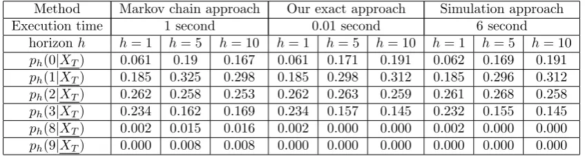
Let us now illustrate how our method fares against the Markov chain approach of McCabe
et al. (2011) and the Monte-Carlo simulation approach of Jung and Tremayne (2006), using a
pre-specified INAR(2) process.10
The following table reports the execution time, as well as the
conditional p.m.f. at horizonsh= 1,5 and10from the three methods, given observations up to timeT.
Method Markov chain approach Our exact approach Simulation approach
Execution time 1 second 0.01 second 6 second
horizonh h= 1 h= 5 h= 10 h= 1 h= 5 h= 10 h= 1 h= 5 h= 10
ph(0|XT) 0.061 0.19 0.167 0.061 0.171 0.191 0.062 0.169 0.191
ph(1|XT) 0.185 0.325 0.298 0.185 0.298 0.312 0.185 0.296 0.312
ph(2|XT) 0.262 0.258 0.253 0.262 0.263 0.259 0.261 0.268 0.258
ph(3|XT) 0.234 0.162 0.169 0.234 0.157 0.145 0.232 0.155 0.145
ph(8|XT) 0.002 0.015 0.016 0.002 0.000 0.000 0.002 0.000 0.000
[image:10.595.87.511.204.317.2]ph(9|XT) 0.000 0.008 0.008 0.000 0.000 0.000 0.000 0.000 0.000
Table 2: Conditional p.m.f. at different horizons obtained by different methods. For expository purpose we have only displayed their values at points0,1,2,3,8 and9.
The reported execution times correspond to the calculation of ph(n|Xt) for horizons h =
1,2, ...,20 and n = 20. For the third approach, the number of simulated paths is equal to
N = 50000. This spells a high computational cost, but is necessary to guarantee the forecasting precision. Indeed, in Table 2 the forecasts provided by our approach and the simulation approach
are quite similar across different horizons, whereas in an unreported comparison where we take
insteadN = 5000as in Jung and Tremayne (2006), we find that the relative error is around 4 percent at horizon 1. As for the Markov chain approximation approach, while at horizon 1, it
provides reliable forecasts, this is no longer the case at higher horizonsh= 5,10. In other words the approximation error accumulates ashincreases and this approach fails to well approximate the long-term behavior of the process, which echos the concerns we raised at the beginning of
Section 4. We do not report the counterpart of this table for an INAR(5) model since i) for this latter model, the Markov chain approach is too costly for a PC ii) the comparison result between our approach and the simulation approach is similar to Table 2, with ours being both
much faster and more precise.
Section 3. Since there are in total(n+ 1)p=O(np)non-zero entries, the total complexity isO(n(p+3)).
10
The parameter values of the model are set to beα1=α2= 0.2, λ= 1, with terminal valuesXT = 3, XT = 5.
5
Concluding remarks
We have solved the open problem that in INAR(p) models, both the likelihood function and multi-step probabilistic forecasts “seem” to be computationally intractable. Our method is based
on i) the simple relationship between the p.g.f. and p.m.f. for a count distribution; ii) the CaR property of the INAR(p) process. Our method eliminates the estimation bias due to the saddlepoint approximation of Pedeli et al. (2015), as well as the approximation (resp. simulation)
error of McCabe et al. (2011) [resp. Jung and Tremayne (2006)] when it comes to forecasting.
Finally, while we have illustrated our methodology for the benchmark INAR(p)model with binomial thinning and Poisson innovation, the same technique can be applied to a large family
of CaR models of the form:
Xt= Xt−1
X i=1
Z1,i,t+1+ Xt−2
X i=1
Z2,i,t+1+· · ·+ Xt−p
X i=1
Zp,i,t+1+ǫt (17)
where Zi,j,t and ǫt are mutually independent, but not necessarily binary/Poisson distributed,
respectively. In this case, for estimation (resp. forecasting), we need to replace, in eqn. (4) [resp.
eqn (11)-(15)], functionslog(αiu+ 1−αi),i= 1, ..., pand/orλ(u−1)by the log p.g.f. functions
ofZi,j,t, andǫt. Thus for the conditional p.m.f. of model (17) to be computable, it suffices that
the two new log p.g.f. are easily Taylor-expanded. For instance, Risti´c et al. (2009); Gouri´eroux
and Lu (2017) assume Zi,j,t and/or ǫt to be negative binomial (or geometric) distributed to
account for conditional over-dispersion,11
, Zhu and Joe (2010) introduce a family of INAR(1)
models such thatZ1,t+1andǫthave Taylor-expandable p.g.f., Schweer and Weiß (2014) consider
compound Poisson distributed innovations, whereas Drost et al. (2009) allowǫtto have a flexible
non-parametric distribution.
Another extention concerns bivariate INAR(p) models. The behchmark bivariate INAR(1) model [see e.g. Pedeli and Karlis (2013)] assumes that:
X1t=α11◦X1t−1+α12◦X2t−1+ǫ1t
X2t=α11◦X1t−1+α12◦X2t−1+ǫ2t 11
The log p.g.f. of a negative binomial distribution with parametersp <1andr >0is equal torlog(1−p)−
rlog(1−pu), which can be Taylor-expanded intorlog(1−p)−r
Pn i=1
1
ip
where αi,j ◦X1,t−1, i, j = 1,2 are conditionally independent and binomial distributed, and
(ǫ1t, ǫ2t)follow a bivariate Poisson distribution. They show that the conditional p.m.f. p(X1t, X2t|Xt−1)
in this model involves a four dimensional summation, and argue that a higher-order generalization
would have an intractable likelihood function. The methodology developed here seems adapted
to this problem, since both the Taylor’s expansion and the theory of CaR process are readily
available in the bivariate case. This is left for future research.
Appendix: Proof of Proposition 2
Let us proceed by induction. Initial conditions (11) and (12) are consequences of Equation (4).
Assume that (10) holds for a certain horizonh, then:
E[uXt+h|X
t−1] =E
h
E[uXt+h|X
t]|Xt−1
i
=E[exphB(h,0)(u) +
p X i=1
B(h, i)(u)Xt+1−i i
|Xt−1]
= exphB(h,0)(u) +
p X i=2
B(h, i)(u)Xt+1−i
i
EhexpB(h,1)(u)Xt|Xt−1
i
(18)
= exphB(h,0)(u) +
p X i=2
B(h, i)(u)Xt+1−i+λ[eB(h,1)(u)−1] + p X i=1
log(αieB(h,1)(u)+ 1−αi)Xt−i i
.
(19)
where in (18) we have used the conditional moment generating function E[etXt|X
t−1]. Its
ex-pression is obtained by replacingubyetin (4). Thus we recover the RHS of (10) and (10) holds
for anyh.
References
Al-Osh, M. and Alzaid, A. A. (1987). First-order Integer-valued Autoregressive (INAR(1))
Pro-cess. Journal of Time Series Analysis, 8(3):261–275.
Statistical Applications. Journal of the Royal Statistical Society. Series B (Methodological), pages 279–312.
Bu, R. and McCabe, B. (2008). Model Selection, Estimation and Forecasting in INAR (p) Models: A Likelihood-based Markov Chain Approach. International Journal of Forecasting, 24(1):151–162.
Bu, R., McCabe, B., and Hadri, K. (2008). Maximum Likelihood Estimation of Higher-Order
Integer-Valued Autoregressive Processes. Journal of Time Series Analysis, 29(6):973–994. Darolles, S., Gourieroux, C., and Jasiak, J. (2006). Structural Laplace Transform and Compound
Autoregressive Models. Journal of Time Series Analysis, 27(4):477–503.
Davies, R. B. (1973). Numerical Inversion of a Characteristic Function. Biometrika, 60(2):415– 417.
Drost, F. C., Akker, R. v. d., and Werker, B. J. (2009). Efficient Estimation of Auto-Regression
Parameters and Innovation Distributions for Semiparametric Integer-Valued AR (p) models.
Journal of the Royal Statistical Society: Series B (Statistical Methodology), 71(2):467–485. Du, J. and Li, Y. (1991). The Integer-Valued Autoregressive (INAR (p)) Model. Journal of Time
Series Analysis, 12(2):129–142.
Gibson, D. and Seneta, E. (1987). Augmented Truncations of Infinite Stochastic Matrices. Jour-nal of Applied Probability, 24(3):600–608.
Gouri´eroux, C. and Lu, Y. (2017). Negative Binomial Autoregressive Process. CREST DP. Jung, R. C. and Tremayne, A. (2006). Coherent Forecasting in Integer Time Series Models.
International Journal of Forecasting, 22(2):223–238.
Knuth, D. E. (1997). The Art of Computer Programming, volume 3. Pearson Education. McCabe, B. P., Martin, G. M., and Harris, D. (2011). Efficient Probabilistic Forecasts for Counts.
Journal of the Royal Statistical Society: Series B (Statistical Methodology), 73(2):253–272. McKenzie, E. (1985). Some Simple Models for Discrete Variate Time Series. Journal of the
Pedeli, X., Davison, A. C., and Fokianos, K. (2015). Likelihood Estimation for the INAR
(p) Model by Saddlepoint Approximation. Journal of the American Statistical Association, 110(511):1229–1238.
Pedeli, X. and Karlis, D. (2013). Some Properties of Multivariate INAR (1) Processes. Compu-tational Statistics & Data Analysis, 67:213–225.
Risti´c, M. M., Bakouch, H. S., and Nasti´c, A. S. (2009). A New Geometric First-order
Integer-valued Autoregressive (NGINAR (1)) Process. Journal of Statistical Planning and Inference, 139(7):2218–2226.
Schweer, S. and Weiß, C. H. (2014). Compound Poisson INAR (1) Processes: Stochastic
Prop-erties and Testing for Overdispersion. Computational Statistics & Data Analysis, 77:267–284. Tweedie, R. (1998). Truncation Approximations of Invariant Measures for Markov Chains.
Jour-nal of Applied Probability, 35(3):517–536.
Zhu, R. and Joe, H. (2010). Negative Binomial Time Series Models Based on Expectation