Negative interest rate policy in a permanent liquidity trap

Munich Personal RePEc Archive

Negative interest rate policy in a

permanent liquidity trap

Murota, Ryu-ichiro

Faculty of Economics, Kindai University

21 April 2019

Online at

https://mpra.ub.uni-muenchen.de/93498/

Negative Interest Rate Policy in a Permanent

Liquidity Trap

Ryu-ichiro Murota

Faculty of Economics, Kindai University

April 21, 2019

Abstract

Using a dynamic general equilibrium model, this paper theoretically analyzes a negative interest rate policy in a permanent liquidity trap. If the natural nominal interest rate is above the lower bound set by the presence of vault cash held by commercial banks, a reduction in the nominal rate of interest on excess bank reserves can get an economy out of the permanent liquidity trap. In contrast, if the natural nominal interest rate is below the lower bound, then it cannot do so, but instead a rise in the rate of tax on vault cash is useful for doing so.

Keywords: aggregate demand, liquidity trap, negative nominal interest rate, unemployment

JEL Classification Codes: E12, E31, E58

∗_{I would like to thank Takayuki Ogawa and Yoshiyasu Ono for helpful comments,}

discussions, and suggestions.

†_{Address: Faculty of Economics, Kindai University, 3-4-1 Kowakae, Higashi-Osaka,}

1

Introduction

Recently, negative interest rate policies have been implemented in Europe

and Japan (see, e.g., Bech and Malkhozov, 2016, and Angrick and Nemoto,

2017). Some economists presented positive views of negative nominal

inter-est rates, but others presented negative views. For example, using Old and

New Keynesian models, Buiter and Panigirtzoglou (2003) showed that paying

negative interest on currency (imposing a carry tax on currency) eliminates

the zero lower bound on nominal interest rates and, hence, is useful for

elimi-nating a liquidity trap.1

Without developing theoretical models, Goodfriend

(2000) suggested a carry tax on bank reserves as a way of overcoming the zero

lower bound, and Fukao (2005) proposed a tax on government-backed

finan-cial assets as a way to get the Japanese economy out of the stagnation that

it has been experiencing since the 1990s. Abo-Zaid and Gar´ın (2016) showed

that the optimal nominal interest rate is negative in a New Keynesian model

with a borrowing constraint. Rognlie (2016) constructed a

money-in-the-utility-function model where the utility of money is saturated and showed

that the optimal interest rate is negative under price rigidity. Meanwhile,

Eggertsson et al. (2019) argued that lowering the nominal rate of interest on

bank reserves to negative values reduces commercial banks’ profits and has

a contractionary effect on output. They developed a New Keynesian model

with a commercial banking sector and examined the effects of a negative

nominal interest rate in a short-run slump caused by a preference shock.

1

It seems that the Euro zone and Japan, where negative interest rate

policies have been implemented, have not been in short-run but long-run

liquidity traps. It is well known that Japan has been in a prolonged liquidity

trap since the 1990s. Recently, there have been concerns that the Euro zone

may also have been in a prolonged liquidity trap. The purpose of this paper

is to theoretically analyze a negative interest rate policy in a permanent

liquidity trap.2

For this purpose, I extend the dynamic general equilibrium

model of Murota and Ono (2012) in two ways. First, I consider that negative

nominal interest is paid on excess bank reserves. In fact, the European

Central Bank and the Bank of Japan have imposed negative nominal interest

on excess reserves (see, e.g., Angrick and Nemoto, 2017). Second, I assume

that a tax is levied on commercial banks’ vault cash holdings in order to

examine the effectiveness of a Gesell tax discussed by Goodfriend (2000),

Buiter and Panigirtzoglou (2003), and Fukao (2005).

As in Murota and Ono (2012), I present a permanent liquidity trap, where

nominal interest rates are stuck at their lower bounds, deficient aggregate

demand creates unemployment, excess bank reserves arise, and the money

multiplier declines. Furthermore, even the price change rate is not in control

of the central bank; that is, deflation can arise despite an increase in the

monetary base. These are the phenomena observed in Japan’s liquidity trap

since the 1990s. In this permanent liquidity trap, I investigate the effects of

2

a reduction in the nominal rate of interest on excess reserves, which is the

policy rate in the present model.

This paper shows that a reduction in the nominal rate of interest on

ex-cess reserves boosts an economy falling into the permanent liquidity trap

to the extent that it lowers the nominal deposit rate. It increases

house-hold consumption (aggregate demand), reduces unemployment, and raises

the price change rate. If the natural nominal interest rate is higher than

the lower bound set by the presence of vault cash, it can lower the nominal

deposit rate to the level of the natural nominal interest rate. Consequently,

the economy gets out of the permanent liquidity trap and reaches a normal

steady state. However, if the natural nominal interest rate is lower than

the lower bound, the economy cannot escape the permanent liquidity trap

no matter how negative the nominal rate of interest on excess reserves

be-comes. This is because the nominal deposit rate reaches the lower bound

and does not go down to the level of the natural nominal interest rate. In

this situation, where lowering the nominal rate of interest on excess reserves

becomes ineffective, instead, a rise in the rate of tax on vault cash is useful

for pulling the economy out of the permanent liquidity trap because it allows

the nominal deposit rate to fall to the level of the natural nominal interest

rate. This is consistent with the suggestions by Goodfriend (2000), Buiter

and Panigirtzoglou (2003), and Fukao (2005). In the present model, however,

levying a tax on currency held by the public, which is practically difficult, is

not required for overcoming the lower bound.

This paper proceeds as follows. Section 2 develops the model of an

a normal steady state as a benchmark. Sections 5 and 6 discuss the effects

of a negative interest rate policy in a permanent liquidity trap. Section 7

concludes this paper.

2

Model

This section extends the dynamic general equilibrium model of Murota and

Ono (2012).3

Excess bank reserves bear nominal interest, which can be

negative. Commercial banks hold vault cash, and a tax is levied on vault

cash holdings. In addition, I provide a microfoundation for nominal wage

stickiness by modifying the fair wage setting of Raurich and Sorolla (2014).

2.1

Household

A representative household derives utility not only from cash but also from

bank deposits.4

The lifetime utility of this household is

∫ ∞

0

[u(ct) +v(mh

t, dt)−ntf(et)] exp(−ρt)dt,

where ρ (> 0) is the subjective discount rate. u(ct) denotes the utility of consumption ct and satisfies

u′

(ct)>0, u′′

(ct)<0, u′

(0) =∞, u′

(∞) = 0. (1)

v(mh

t, dt) denotes the utility of real cash holdings mht (≡ Mth/Pt) and real deposit holdings dt (≡ Dt/Pt), where Mth is nominal cash holdings, Dt

3

Murota and Ono (2012) did not consider vault cash or interest paid on bank reserves and assumed nominal wage stickiness without microfoundations.

4

is nominal deposit holdings, and Pt is the price level. v(mht, dt) is linear homogeneous and satisfies

∂v ∂mh

t

≡vm(mh

t, dt)>0,

∂2

v ∂mh t

2 <0, vm(0, dt) =∞, vm(∞, dt) = 0;

∂v ∂dt

≡vd(mh

t, dt)>0,

∂2

v ∂dt

2 <0, vd(m

h

t,0) =∞, vd(mht,∞) = 0.

The cash–deposit ratio is defined by xt:

xt≡

mh t

dt

. (2)

Then the marginal utility of cash and of deposits are expressed as functions

of xt:

vm(mht, dt)≡vm(xt), vd(m h

t, dt)≡vd(xt), and the above-mentioned properties of v(mh

t, dt) are rewritten as follows:

v′

m(xt)<0, vm(0) =∞, vm(∞) = 0;

v′

d(xt)>0, vd(0) = 0, vd(∞) =∞.

(3)

−ntf(et) denotes the disutility of effort, where nt is the amount of em-ployed labor, et is effort per unit of employed labor, and −f(et) is the disu-tility of effort per unit of employed labor. Following Raurich and Sorolla

(2014), I assume a quadratic disutility function:5

−ntf(et) =−nt [

et−e(Wt/WtR) ]2

,

where Wt is the nominal wage, WtR is the nominal reference wage, and

e(Wt/WtR) is the norm of effort and where the household takes nt, Wt, and

WR

t as given. Furthermore, following them, I assume that the reference wage 5

is given by the weighted average of past social averages of income. However,

unlike them, the reference wage consists of nominal wages, not real wages,

as follows:

WR t ≡

∫ t

−∞

Isαexp(−α(t−s))ds, (4)

where α is a positive constant and where Is is the social average of nominal income defined such that

Is ≡

Wsns+βWs(nf −ns)

nf , (5)

where nf _{is the labor endowment that the household inelastically supplies,}

nf_−n

sis unemployment, andβWs(nf−ns) is unemployment benefits received by the household (β is the replacement rate satisfying 0< β <1).

The budget constraint in real terms is

˙

at=rDt dt−πtmht +wtnt+βwt(nf −nt)−ct−st, (6)

where at is real asset holdings, rtD is the real rate of interest on deposits,

πt (≡ P˙t/Pt) is the rate of price change, wt (≡ Wt/Pt) is the real wage, and

stis a lump-sum tax or transfer. The components ofatare cash and deposits:

at=mht +dt. (7)

The current-value Hamiltonian H_{t for the utility-maximization problem}

is

H_{t=u(ct) +v(m}h_{t, dt)−nt}[_et−e(Wt/WtR₎]2

+λt [

rD

t dt−πtmht +wtnt+βwt(nf −nt)−ct−st ]

+γt (

at−mht −dt )

where λt is the costate variable associated with (6) and γt is the Lagrange multiplier associated with (7). The first-order conditions with respect to ct,

mh

t,dt, at, and et are

u′

(ct) = λt,

vm(xt)−πtλt=γt,

vd(xt) +rD

t λt=γt, ˙

λt−ρλt=−γt,

et=e(Wt/WtR).

(8)

The transversality condition is

lim

t→∞λtatexp(−ρt) = 0. (9)

The last equation of (8) shows that in contrast with Raurich and Sorolla

(2014), effort et depends on nominal wages (not real wages).

6

I assume that

e′

(Wt/WtR)>0, e

′′

(Wt/WtR)<0.

The assumption that e′

(·)>0 implies that as a firm pays a higher nominal wage compared with the nominal reference wage (which is the criterion for

judging fairness), the household provides greater effort in return. There

are empirical findings consistent with this assumption. Kahneman et al.

(1986) and Blinder and Choi (1990) found evidence of money illusion that

people tend to judge fairness in terms of nominal wages. Shafir et al. (1997)

and Mees and Franses (2014) also found evidence of money illusion that

nominal wages tend to influence worker morale. Moreover, Campbell and

Kamlani (1997), Bewley (1999), and Kawaguchi and Ohtake (2007) found

6

that reductions in nominal wages decrease worker morale. The assumption

that e′′

(·)<0 is required for the second-order condition for the firm’s profit-maximization problem. See Murota (2016) for a somewhat similar effort

function where effort depends on nominal wages because of money illusion.

From (8) except the last equation, I obtain

ρ+η(ct)c˙t

ct

+πt =

vm(xt)

u′_(ct) =R

D t +

vd(xt)

u′_(ct), (10)

where η(ct) ≡ −u′′

(ct)ct/u′(ct) and RDt (≡ rDt +πt) is the nominal rate of interest on deposits. According to (10), the household decides to consume or

save and allocates wealth between cash and deposits. Equation (10) implies

that even when the nominal deposit rate RD

t is negative, the marginal utility of cash vm(·) can be positive owing to the presence of the marginal utility of deposits vd(·). This makes equilibrium with negative nominal interest rates feasible.

2.2

Firm

The production function of a representative firm is linear as follows:

yt=etnt=e(Wt/WtR)nt, (11)

where yt is output, effort et is labor productivity, andnt is labor input. The firm chooses nt and Wt to maximize its profit:

Pte(Wt/WtR)nt−Wtnt,

av-erages of income. The first-order conditions with respect to nt and Wt are7

e(Wt/WtR) =

Wt

Pt

, (12)

Pte

′

(Wt/WtR)

WR t

= 1. (13)

Eliminating Pt from (12) and (13) yields a modified Solow condition:

(Wt/WtR)e

′

(Wt/WtR)

e(Wt/WtR)

= 1, (14)

which gives Wt/WtR as a constant. Denoting it byω:

Wt

WR t

≡ω, (15)

I find that effort (labor productivity) is constant:

et =e(Wt/WtR) = e(ω)≡e. (16)

2.3

Commercial Bank

A representative commercial bank collects deposits Dt from the household and buys government bondsBt, which bears nominal interest at the rateRB

t . In this regard, however, the commercial bank is required to put an amount

of money greater than or equal to a portion of the deposits in the central

bank as bank reserves:

Mtb ≥ϵDt, (17) 7

Under the linear production technology, the firm chooses labor input and output as follows:

nt=∞, yt=∞ if e(Wt/WtR)> Wt/Pt,

0< nt<∞, 0< yt<∞ if e(Wt/WtR) =Wt/Pt,

nt= 0, yt= 0 if e(Wt/WtR)< Wt/Pt.

Since Wt is determined by the firm so as to satisfy (13), Pt flexibly falls (rises) so as to

eliminate excess supply (excess demand) in the perfectly competitive goods market when

whereMb

t is bank reserves (commercial bank’s deposits with the central bank)

and ϵ is the required reserve ratio (0 < ϵ < 1). Unlike Murota and Ono (2012), I consider that excess reserves (Mb

t −ϵDt) bear nominal interest at the rate R, which is the policy rate and an exogenous variable controlled by the central bank. In the present model, a negative interest rate policy

indicates the case of

R <0.

Moreover, unlike them, I take into consideration vault cash. Besides Bt and

Mb

t, the commercial bank can hold vault cash Zt:

Zt ≥0. (18)

Naturally, the nominal rate of interest on vault cash is zero. In sum, the

following relationship holds:

Bt+Mtb+Zt =Dt. (19)

The relationship between bank reserves and vault cash varies in different

countries. For example, in Japan, vault cash is not included in bank reserves

(bank reserves consist only of commercial banks’ deposits with the Bank of

Japan),8

which means that (17) holds. In contrast, in the USA, both vault

cash and deposits with Federal Reserve Banks are included in bank reserves,9

which means that the equationMb

t +Zt≥ϵDtholds instead of (17). I adopt (17) because Japan is the country that has implemented a negative interest

rate policy.10

8

See http://www.boj.or.jp/en/announcements/education/oshiete/seisaku/b33.htm/.

9

See https://www.federalreserve.gov/monetarypolicy/reservereq.htm.

10

The commercial bank’s profit-maximization problem is as follows:

maxRB

t Bt+R(Mtb−ϵDt)−τ Zt−RtDDt, s.t. Mb

t ≥ϵDt, Zt≥0, Bt+Mtb+Zt=Dt,

where τ is the rate of tax on vault cash. The presence of the cost of holding vault cash plays an important role in considering negative nominal interest

rates. Given RB

t and RtD, the commercial bank chooses Bt, Mtb, Zt, and

Dt to maximize its profit. The Lagrange function Lt for this maximization problem is

L_t=RB_{t Bt+R(Mt}b_{−ϵDt)−τ Zt−R}D_{t Dt}

+κt(Mb

t −ϵDt) +ξtZt+δt(Dt−Bt−Mtb−Zt),

where κt, ξt, and δt are the Lagrange multipliers associated with (17), (18), and (19), respectively. The first-order conditions are

RB t =δt,

R+κt=δt,

−τ+ξt=δt,

RD

t =δt−ϵ(R+κt),

κt≥0, Mtb−ϵDt≥0, κt(Mtb−ϵDt) = 0,

ξt≥0, Zt≥0, ξtZt= 0.

(20)

From (20), I obtain

RB

t ≥R, Mtb−ϵDt≥0, (RBt −R)(Mtb−ϵDt) = 0,

RB

t ≥ −τ, Zt ≥0, (RBt +τ)Zt = 0.

From (21), the lower bound onRB

t is given by the high side ofRand −τ:

11,12

RB

t ≥max{R,−τ}, (22)

which implies that the lower bound is created by the presence of excess

reserves and vault cash.

In what follows, I consider the case of

R > −τ. (23)

The case of R <−τ is analyzed later in Section 6. In the case of (23), from (22), the lower bound on RB

t is R:

RB

t ≥R >−τ,

which means that vault cash is less profitable than government bonds and

excess reserves. Therefore, as is clear from (21), the commercial bank does

not hold vault cash:

Zt = 0, (24)

i.e., (18) is binding (ξt>0).

In the case of (23), in contrast with (18), (17) is either binding or

non-binding. When (17) is binding (κt >0), i.e., the commercial bank does not hold excess reserves:

Mtb =ϵDt, (25)

11

If RB

t < max{R,−τ} (government bonds are less profitable than excess reserves or

vault cash), the commercial bank by no means buys government bonds. In this case,

RB

t rises to a level higher than or equal to max{R,−τ} so that the government gets the

commercial bank to buy bonds. Consequently, (22) holds.

12

In Murota and Ono (2012), whereR=τ = 0, the lower bound onRB

from (20) I obtain

RBt > R, R D

t = (1−ϵ)R B

t >(1−ϵ)R (26)

and from (19), (24), and (25) I get

Dt =

Bt 1−ϵ, M

b t =

ϵ

1−ϵBt. (27)

Meanwhile, when (17) is not binding (κt = 0), i.e., the commercial bank holds excess reserves:

Mb

t −ϵDt>0, from (20) I obtain

RB

t =R, R D

t = (1−ϵ)R B

t = (1−ϵ)R. (28)

In other words, excess reserves arise when the return on excess reserves equals

that on government bonds. From (26) and (28), I find that independently

of whether (17) is binding (excess reserves arise), the following relationship

holds:

RtD = (1−ϵ)R B

t , (29)

where the left-hand side (LHS) and the right-hand side (RHS) denote the

marginal cost of and the marginal revenue of collecting deposits, respectively,

and that the lower bound on RD

t is (1−ϵ)R:

RDt ≥(1−ϵ)R.

Note that from (24), (26), and (27) or from (19), (24), and (28) the profit of

the commercial bank is zero:

RB

2.4

Government and Central Bank

Besides controlling the nominal rate of interest on excess reserves,R, the cen-tral bank increases or decreases the nominal monetary baseMt at a constant rate µ:

˙

Mt

Mt =µ,

which implies that the real monetary base mt (≡ Mt/Pt) evolves according to

˙

mt

mt

=µ−πt. (31)

The budget constraint of the government in nominal terms is

˙

Bt+ ˙Mt+Ptst+τ Zt−R(Mtb−ϵDt) = R B

t Bt+βWt(nf −nt) +Ptg,

where g is government purchases and where −R(Mb

t −ϵDt) denotes the gov-ernment revenue arising from negative interest on excess reserves whenR <0. In real terms, it is

˙

bt+µmt+st+τ zt−R(mbt−ϵdt) = r B

t bt+βwt(nf −nt) +g, (32)

where bt (≡Bt/Pt) is real government bonds, zt (≡Zt/Pt) is real vault cash holdings, mb

t (≡Mtb/Pt) is real reserve holdings, and rtB (≡RBt −πt) is the real rate of interest on government bonds. To prevent bt from diverging, the government collects the lump-sum tax st according to

st =rtBbt+βwt(nf −nt) +g+R(mbt−ϵdt)−τ zt−µmt+ϕ(bt−b),

where ϕ is a positive constant and b is the target level of real government bonds. Substituting this equation into (32) yields the law of motion for bt:

˙

3

Dynamics

This section derives the dynamic system of the economy. From (4), (5), and

(15), the nominal wage changes according to13

˙

Wt

Wt = W˙

R t WR t =α ( It WR t −1 ) =α (

ω(1−β)nt+βωnf

nf −1 )

=σ

(

nt−n

nf )

,

(34)

where σ and n are positive constants defined such that

σ≡αω(1−β), n≡

[

1−βω ω(1−β)

]

nf _{< n}f_,

where the inequality is established by the assumption that ω > 1.14

From

(34), I find15

d( ˙Wt/Wt)

dnt

= σ

nf >0,

which is produced as follows. An increase in employment nt leads to an increase inIt/WtRand, hence, to a rise in ˙WtR/WtR. This rise in the reference wage puts downward pressure on effort (∂e(Wt/WtR)/∂WtR <0). Since the

13

Murota (2016, 2018) derived nominal wage stickiness similar to (34) in a discrete time model where worker morale depends on the current and last nominal wages and on the unemployment rate and in a model where labor unions are concerned about nominal wages and employment, respectively.

14

For example, if the effort function is logarithmic:

e(Wt/WtR) = ln(Wt/WtR),

then from (14) the assumption thatω >1 is satisfied:

ω= e = 2.71828· · ·>1.

15

The rate of change in the nominal wage ˙Wt/Wtis related negatively to the

unemploy-ment rate (nf_−n

t)/nf (i.e., a Phillips curve appears):

˙

Wt

Wt

=−σ

(

nf_−n t

nf )

+σ

(

nf_−n

nf )

firm raises the nominal wage in order to maintain labor productivity at the

optimal level, ˙Wt/Wt rises at the same rate as ˙WtR/WtR.

In the case of (23), where the commercial bank does not hold vault cash

(see (24)), the money market equilibrium condition is

mht +m b

t =mt. (35)

Supply equals demand in the goods market as follows:16

ct+g =yt=ent. (36)

From (12), (16), (34), and (36), the price change rate is

πt= ˙

Wt

Wt =σ

(

nt−n

nf )

=σ

(

ct+g−y

yf )

, (37)

where

y≡en, yf _≡enf_{, (38)}

where yf _{denotes full employment output. From (31) and (37), the law of} motion for mt is

˙

mt

mt

=µ−πt =µ−σ (

ct+g−y

yf )

. (39)

From the first equality of (10) and (37), the law of motion forct is

˙

ct

ct

=η(ct)−1

[

−σ

(

ct+g−y

yf )

+vm(xt)

u′_(ct) −ρ

]

. (40)

When (17) is binding (the commercial bank does not hold excess reserves),

from (2), (27), and (35), xt in (40) is expressed by bt and mt:

xt=

mh t

dt

= (1−ϵ)mt

bt

−ϵ. (41)

16

When (17) is not binding (the commercial bank holds excess reserves), from

the second equality of (10) into which (28) is substituted:

vm(xt)

u′

(ct) = (1−ϵ)R+

vd(xt)

u′

(ct), (42)

xt in (40) is given as a function of ct and R:

xt=x(ct;R), (43)

which satisfies17

x(0;R) = ∞ if R <0, x(0;R) =x if R= 0, x(0;R) = 0 if R >0, (44)

where x is a value satisfying vm(x) =vd(x). In addition, xt satisfies

18

∂xt

∂ct

<0 if R <0, ∂xt ∂ct

= 0 if R = 0, ∂xt ∂ct

>0 if R >0; (45)

∂xt

∂R =

(1−ϵ)u′

(ct)

v′

m(xt)−v

′

d(xt)

<0, (46)

where the inequality of (46) is established by (1) and (3). In sum, the dynamic

system consists of (33), (39), and (40) with (41) or (43).

17

Arranging (42) yields

vm(xt)−vd(xt)

u′_(c

t)

= (1−ϵ)R,

where the RHS is a finite constant and the denominator of the LHS is infinity whenct= 0

(u′_{(0) = ∞ from (1)). IfR < 0, for the equality to be satisfied, then the numerator of}

the LHS must be minus infinity when ct = 0. Therefore, when ct = 0, from (3) I have

xt = ∞ (the numerator is vm(∞)−vd(∞) = 0− ∞= −∞). IfR > 0, I have xt = 0

(vm(0)−vd(0) =∞) because the numerator of the LHS must be plus infinity.

18

From (42), I derive

∂xt

∂ct

= u

′′_(c

t) [vm(xt)−vd(xt)]

u′_(c

t) [v′m(xt)−v′d(xt)]

= (1−ϵ)Ru

′′_(c

t)

v′

m(xt)−vd′(xt)

.

4

Normal Steady State

Prior to dealing with a permanent liquidity trap, in this section, I consider

a normal steady state, where the nominal interest rates RB _{and R}D _are above the lower bounds R and (1−ϵ)R, respectively, and where there is no aggregate demand deficiency. From (33), (39), and (40) where ˙bt = 0,

˙

mt= 0, and ˙ct= 0, the normal steady state is represented by

b∗

=b, µ=π∗

=σ

(

c∗

+g−y yf

)

, ρ+µ= vm(x

∗

)

u′

(c∗

) , (47) where the asterisk is attached to endogenous variables. Throughout this

paper, I assume that µ > −ρ. The existence of this steady state is easily shown. The real bond b∗

and the price change rate π∗

are straightforwardly

determined by the first and second equations of (47). From (36), (38), and

the second equation of (47), consumption and employment are

c∗

= µ

σy

f _{+y−g, n}∗

= µ

σn

f _{+n. (48)}

The second equation of (48) implies the existence of unemployment as follows:

nf _−n∗

>0 if µ < σ

(

nf _−n

nf )

.

Moreover, from (48), I find a crowding-out effect of government purchasesg:

dc∗

dg =−1, dn∗

dg = 0,

which implies that there is no aggregate demand deficiency, i.e., the efficiency

wage is the only cause of unemployment in the normal steady state.

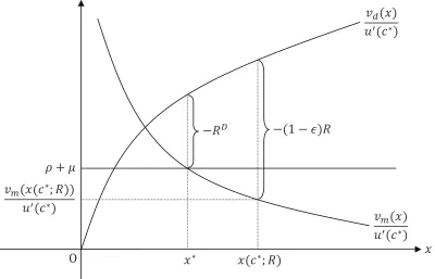
As shown in Figure 1, when

ρ+µ > vm(x(c ∗

;R))

u′

(c∗

where from (42) and (43) x(c∗

;R) is the cash–deposit ratio when c = c∗

and RD _{= (1−ϵ)R, the cash–deposit ratio x}∗

in the last equation of (47) is

determined so as to satisfy

x∗

< x(c∗

;R), (50)

and the nominal deposit rate RD _{is determined so as to be higher than its} lower bound (1−ϵ)R:

(

vm(x∗

)

u′_(c∗₎ − vd(x∗

)

u′_(c∗₎ =

)

RD _>(1−ϵ)R (

= vm(x(c

∗

;R))

u′_(c∗₎ −

vd(x(c∗

;R))

u′_(c∗₎

)

,

(51)

which straightforwardly results from −RD _{<−(1−ϵ)R in Figure 1.}19

Note

that the equalities of (51) are obtained from the second equality of (10) and

that the properties of vm(x) andvd(x) in (3) yield (50) and (51) under (49). From (29) and (51), the government bond rate RB _{is determined so as to be} higher than its lower bound R and is defined byR∗

:

R < R

D 1−ϵ =R

B _≡R∗

. (52)

Then RD _{is expressed as}

RD _{= (1−ϵ)R}∗ .

Thus, in the normal steady state, the optimality condition of the household,

(10), holds as follows:

ρ+µ= vm(x

∗

)

u′

(c∗

) = (1−ϵ)R

∗

+ vd(x

∗

)

u′

(c∗

). (53)

Since R∗

and (1−ϵ)R∗

are the nominal interest rates that hold in the

normal steady state where RB _{and R}D _{are higher than their lower bounds} 19

and where aggregate demand is not deficient, I regard R∗

and (1 − ϵ)R∗

as natural nominal interest rates. In the present model, nominal interest

rates rather than real interest rates are important because the cash–deposit

ratio, which is affected by the nominal deposit rate (not the real deposit

rate), plays a crucial role in determining whether the economy falls into a

permanent liquidity trap (see Section 5). From (48) and (53), R∗

is given by

R∗

= vm(x

∗

)−vd(x∗

)

(1−ϵ)u′

(µ

σy

f _+y−g), (54)

where x∗

is

x∗

=v−1

m (

(ρ+µ)u′(µ σy

f _+y−g))_{. (55)}

From (54) and (55), I find that R∗

is independent of the nominal rate of

interest on excess reserves, R, and the rate of tax on vault cash, τ, and that if ρ, σ, and g are sufficiently small and yf _{and y are sufficiently large, then} the natural nominal interest rate is negative:20

R∗ <0.

Moreover, R∗

has the following property.

Lemma 1. Equation (49) is necessary and sufficient for (52).

20

From (55), I obtain

∂x∗

∂ρ = u′

v′

m

<0, ∂x

∗

∂σ =−

µyf_(ρ+µ)u′′

σ2_v′

m

<0, ∂x

∗

∂g =−

(ρ+µ)u′′

v′

m

<0,

∂x∗

∂yf =

µ(ρ+µ)u′′

σv′

m

>0, ∂x

∗

∂y =

(ρ+µ)u′′

v′

m

>0.

Hence, from (3) and (54), I have R∗ _{<0 ifρ,σ, and g are sufficiently small and y}f _and

y are sufficiently large. Note that the influence of µonR∗ _{is unclear because the sign of}

∂x∗_{/∂µ is ambiguous: ∂x}∗_{/∂µ= [σu}′_{+ (ρ+µ)y}f_u′′_]/(σv′

Proof. Since from (3)vm(x) is a monotonically decreasing function ofx, using the last equation of (47), I find

(49) ⇐⇒ (50).

Taking into account that from (3)vm(x)−vd(x) is a monotonically decreasing function of x, I have

(50) ⇐⇒ (51).

Thus, (49) is necessary and sufficient for (51). Since (51) is equivalent to

(52), I obtain

(49) ⇐⇒ (52).

I formally state the existence of the normal steady state in the following

proposition.

Proposition 1. When (23) and (52) hold:

R >−τ, R < R∗ ,

there exists the normal steady state represented by (47).

In the normal steady state, where RB _{= R}∗

> R, from (21) excess reserves do not arise (MB _{= ϵD), which implies that the money multiplier is larger} than one:

Mh_+D

M =

(mh_{/d) + 1} (mh_{/d) + (m}b_/d) =

x∗

+ 1

x∗_+ϵ >1.

Now, I investigate the effects of monetary policies in the normal steady

consumption, employment, and the price change rate:

dc∗ dµ =

yf

σ >0, dn∗

dµ = nf

σ >0, dπ∗

dµ = 1>0,

where the effects of a rise in µonc∗

and n∗

become stronger as the nominal

wage becomes more sticky (i.e., σ decreases). This implies that the cause of the increases in c∗

and n∗

is nominal wage stickiness. Meanwhile, from (47)

and (48), I obtain the following proposition.

Proposition 2. A change in the nominal rate of interest on excess reserves,

R, does not affect consumption, employment, or the price change rate:

dc∗ dR = 0,

dn∗ dR = 0,

dπ∗ dR = 0.

The reason for this ineffectiveness is that the nominal deposit rateRD _{is not} affected by a change in R (RD _{is not stuck at the lower bound (1−ϵ)R).}

5

Permanent Liquidity Trap

This section considers the case where the household’s desire for savings is so

excessive that (49) is not true:

ρ+µ < vm(x(c ∗

;R))

u′_(c∗₎

(

= (1−ϵ)R+vd(x(c

∗

;R))

u′_(c∗₎

)

, (56)

i.e., the natural nominal interest rate is so low that (52) is not true:

R > R∗

. (57)

Note that as inferred from Lemma 1, (56) is necessary and sufficient for (57).

Point A in Figure 2 to be attained), the equation −RD _{> −(1−ϵ)R must} hold, i.e., the nominal deposit rate must be below its lower bound:

RD _<(1−ϵ)R.

Naturally, this is infeasible. Hence, it turns out that under (56) the normal

steady state does not exist. Then, what is the state that the economy reaches

if (56) is true?

Equation (56) implies that the household prefers saving cash and deposits

to consuming when c= c∗

, RD _{= (1−ϵ)R, and x =x(c}∗

;R).21

This desire

for savings is not suppressed by a decline in the nominal deposit rate (the

consequent rise in the cash–deposit ratio) because the nominal deposit rate

already reaches the lower bound (1− ϵ)R (the cash–deposit ratio already reaches the upper bound x(c∗

;R)).22

Thus, in contrast with (53) in the

normal steady state, the optimality condition of the household, (10), is not

satisfied by the adjustment of the nominal deposit rate and the cash–deposit

ratio. A reduction in consumption is required for satisfying (10). That

is, the ungratified desire to save cash and deposits causes the household to

decrease consumption to less than c∗

. This consumption deficiency creates

unemployment. Consequently, the economy reaches a stagnation steady state

where the nominal interest ratesRB _andRD _{are stuck at the respective lower} bounds R and (1−ϵ)R, consumption (aggregate demand) is deficient, and unemployment worsens. In addition, as described below, an increase in the

21

In (56),ρ+µintuitively denotes the degree of preference for consumption. Naturally, higherρcauses the household to save less and consume more. Also higherµ, which means higherπ∗ _whenc=c∗_{, urges the household to consume more because it implies a fall in}

the price of the present good relative to the price of the future good.

22

From (46), a decline in the nominal deposit rate RD _{(= (1−ϵ)R) leads to a rise in}

monetary base is ineffective (even the price change rate is not affected),

excess reserves arise, and the money multiplier decreases to one. In short,

the economy falls into a permanent liquidity trap. From (33), (39), and (40)

with (43), this permanent liquidity trap is represented by

b =b, m˙

m =µ−π=µ−σ

(

c+g−y yf

)

>0, ρ+σ

(

c+g−y yf

)

= vm(x(c;R))

u′_(c) ,

(58)

where

c < c∗

, RB =R, RD = (1−ϵ)R.

Recall that from (28), (42), and (43)RB _{and R}D _{areR and (1−ϵ)R,} respec-tively, when the cash–deposit ratio is x(c;R).

Let me examine the existence of this permanent liquidity trap. As in the

normal steady state, from the first equation of (58), the real bond b is given byb. Meanwhile, consumptioncis determined by the last equation of (58) so as to be lower than the level of the normal steady state c∗

as follows. Using

the first equation of (48) and (56), I find that in the last equation of (58) the

LHS is smaller than the RHS at c=c∗

:

ρ+σ

(

c∗

+g−y yf

)

=ρ+µ < vm(x(c ∗

;R))

Therefore, if the LHS is larger than the RHS at c= 0:23

ρ+σ

(

g−y yf

)

>0 if R≤0, ρ+σ

(

g−y yf

)

>(1−ϵ)R if R >0, (59)

at least one value ofcsatisfying the last equation of (58), denoted by ˜c, exists between 0 and c∗

:

0<˜c < c∗ .

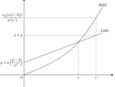
Furthermore, if the slope of the LHS is smaller than that of the RHS at

c= ˜c:24

σ yf <

v′

m(x(˜c;R))

u′

(˜c) ·

∂x(˜c;R)

∂c˜ −

vm(x(˜c;R))u′′

(˜c) [u′

(˜c)]2 ≡f(˜c;R), (60)

then ˜c is unique (Figure 3 illustrates the unique existence of ˜c in the case of R ≤ 0).25

Hence, in contrast with (53) in the normal steady state, the

optimality condition of the household, (10), holds as follows:

ρ+σ

( ˜

c+g−y yf

)

= vm(x(˜c;R))

u′

(˜c) = (1−ϵ)R+

vd(x(˜c;R))

u′

(˜c) . (61)

Using (36) and (37), I find that the consumption deficiency (˜c < c∗

) makes

employment ˜n and the price change rate ˜π in the permanent liquidity trap

23

Whenc= 0, from (1), (3), (42), (43), and (44), the RHS of (58) is

vm(x(0;R))

u′₍₀₎ = 0 if R≤0,

vm(x(0;R))

u′₍₀₎ = (1−ϵ)R if R >0,

where

vd(x(0;R))

u′₍₀₎ =−(1−ϵ)R >0 if R≤0,

vd(x(0;R))

u′₍₀₎ = 0 if R >0.

24

From (1), (3), and (45), whereas the first term of f(˜c;R) is positive if R < 0, it is negative if R > 0 and vanishes if R = 0. However, the second term is always positive, which allows f(˜c;R) to satisfy the inequality of (60) even ifR≥0.

25

lower than the levels of the normal steady state:

˜

n= ˜c+g

e < c∗

+g e =n

∗

, π˜ =σ

( ˜

c+g−y yf

)

< σ

(

c∗

+g−y yf

) =π∗

=µ.

(62)

The first equation of (62) implies that unemployment in the permanent

liq-uidity trap is nf _{−n˜, which is the sum of unemployment created by the} consumption deficiency, n∗

−n˜, and unemployment created by the efficiency wage, nf_−n∗

. The second equation of (62) implies that ˜π can be positive or negative and that the real monetary base permanently increases (m = ∞), as shown by the second equation of (58).26

Taking m = ∞ into account, from (2), (19), (24), and (35), I find that real cash holdings mh_{, real deposit} holdings d, and real bank reserves mb _{also increase to infinity:}

mh ₌ x(˜c;R)(m+b)

1 +x(˜c;R) =∞, d=

m+b

1 +x(˜c;R) =∞, m

b ₌ m−x(˜c;R)b 1 +x(˜c;R) =∞.

(63)

Although household’s wealth holdings increase to infinity (a =mh_+d=∞), household consumption remains insufficient (c = ˜c < c∗

). This is why the

liquidity trap is permanent. I summarize the above discussion in the following

proposition.

26

From (7), the first equation of (8), (19), (24), (35), and (58), I obtain

at=mt+bt, lim t→∞λt=u

′_{(˜c), lim}

t→∞bt=b, tlim→∞

( ˙ mt mt −ρ )

=µ−vm(x(˜c;R))

u′_(˜c) .

Therefore, whenµis so low as to satisfy

µ < vm(x(˜c;R)) u′_(˜c) ,

the rate of growth in mtis lower thanρ, and the transversality condition (9) is satisfied:

lim

t→∞λtatexp(−ρt) =u

′_(˜c)[_lim

t→∞mtexp(−ρt) + limt→∞btexp(−ρt)

]

Proposition 3. When (23) and (57) hold:

R >−τ, R > R∗ ,

there exists the permanent liquidity trap represented by (58).

In this liquidity trap, from (21), excess reserves appear (Mb _{−ϵD > 0)} because the government bond rate equals the nominal rate of interest on

excess reserves (RB _{= R). The presence of excess reserves decreases the} money multiplier to one:

Mh_+D

M =

(mh_{/d) + 1}

(mh_{/d) + (m}b_/d) = 1, where from (63) the reserve–deposit ratio is

mb

d = limm→∞

1−(x(˜c;R)b/m) 1 + (b/m) = 1.

The effects of fiscal and monetary policies in the permanent liquidity

trap are in contrast to those in the normal steady state. From (60), the

first equality of (61), and (62), an increase in government purchases g raises consumption, employment, and the price change rate:

d˜c dg =

σ/yf

f(˜c;R)−(σ/yf₎ >0,

dn˜

dg =

1

e

(

d˜c dg + 1

)

>0, dπ˜ dg =

σ yf

(

d˜c dg + 1

)

>0.

The reason why an increase in government purchases boosts consumption is

that it raises the price change rate (it lowers the price of the present good

relative to the price of the future good). Hence, if the price is fixed (σ = 0), the effect of g vanishes (d˜c/dg= 0). In contrast with an increase in g, from the first equality of (61) and (62), a rise in the money growth rate µhas no effect:

d˜c dµ = 0,

dn˜

dµ = 0, dπ˜

It is noteworthy that even the price change rate is not affected, which implies

that deflation (˜π < 0) can arise despite a monetary expansion (µ >0). See Ono and Ishida (2014) and Murota (2016, 2018) for similar effects of fiscal

and monetary expansions in stagnation steady states.

Whereas a rise inµis ineffective, a change in the nominal rate of interest on excess reserves, R, affects the economy. Totally differentiating the first equality of (61) yields

d˜c dR =−

v′

m(x(˜c;R))

u′_(˜c) ·

∂x(˜c;R)

∂R

[

f(˜c;R)− σ

yf ]−1

<0,

where the inequality is established by (1), (3), (46), and (60). Hence, from

(62), I obtain

dn˜

dR =

1

e · dc˜

dR <0, dπ˜

dR = σ yf ·

dc˜

dR <0.

I restate this result in the following proposition.

Proposition 4. In the permanent liquidity trap, where RD _{is stuck at (1−}

ϵ)R, a reduction in the nominal rate of interest on excess reserves, R, in-creases consumption, employment, and the price change rate.

This proposition is produced through the following mechanism. Since a

re-duction in RlowersRD _{(= (1−ϵ)R), the household is encouraged to shift its} portfolio from deposits to cash (from (46) a reduction in R raises the cash– deposit ratiox(˜c;R)). The rise inx(˜c;R) works to lower the marginal utility of cash vm(x(˜c;R)) (i.e., it works to gratify the household’s desire to hold cash). This causes the household to increase consumption, and the increase

in consumption (aggregate demand) leads to increases in employment and

Note that naturally, in this permanent liquidity trap, a rise in the rate of

tax on vault cash, τ, does not have any effects on consumption, employment, or the price change rate. From (61) and (62), I have

d˜c dτ = 0,

dn˜

dτ = 0, dπ˜

dτ = 0.

Before going on to the next section, I summarize Propositions 1 and 3

in Figure 4. In Region (A) consisting of R > −τ and R < R∗

, the normal

steady state exists. In Region (B) consisting of R > −τ and R > R∗

, the

permanent liquidity trap appears. If R is lowered from Point A to Point B in Figure 4, the economy moves from the permanent liquidity trap to the

normal steady state. Then, if Ris lowered from Point C to Point D in Figure 4, what state does the economy reach? To answer this question, in the next

section, I analyze the case of

R < −τ.

6

Ineffectiveness of Negative Interest Rate

Policy

This section first derives the dynamic system in the case of R < −τ. It then shows that the normal steady state also exists in Region (A) composed

of R < −τ and R∗

> −τ in Figure 5 and that there exists the permanent liquidity trap, whereRD _{is stuck not at (1−ϵ)R but at−(1−ϵ)τ, in Region} (C) composed ofR <−τ andR∗

<−τ in Figure 5. Moreover, it investigates the effects of a fall in R and a rise in τ.

IfR <−τ, from (22), the lower bound on RB

t is −τ (not R):

RB

Since the return on excess reserves is lower than that on government bonds

(R < RB

t ), from (21), the commercial bank does not hold excess reserves:

Mb

t −ϵDt= 0.

Moreover, from (21), the following two cases are possible:

RB

t >−τ and Zt= 0,

RB

t =−τ and Zt>0.

In the case where the government bond rate is higher than its lower

bound (RB

t >−τ) and where the commercial bank does not hold vault cash (Zt = 0), from (20) where κt > 0 and ξt > 0, the nominal deposit rate is higher than −(1−ϵ)τ:

RD

t = (1−ϵ)RBt >−(1−ϵ)τ. (64)

In this case, because of Zt = 0 and Mtb −ϵDt = 0, the dynamic system is given by (33), (39), and (40) with (41).

In the case where the government bond rate is stuck at its lower bound

(RB

t = −τ) and where the commercial bank holds vault cash (Zt > 0), the money market equilibrium condition (35) is modified as follows:

mht +m b

t+zt=mt, (65)

whereztis real vault cash holdings. However, the law of motion ofmtremains (39). Meanwhile, the law of motion of ct, (40), is modified; the cash–deposit ratio xt is no longer (41) or (43) as follows. In the case of RBt = −τ and

Zt >0, from (20) where κt> 0 and ξt = 0, the nominal deposit rate equals

−(1−ϵ)τ:

RD

t = (1−ϵ)R B

From the second equality of (10) with (66):

vm(xt)

u′

(ct) =−(1−ϵ)τ+

vd(xt)

u′

(ct),

xt in (40) is given by a function of ct and −τ:

xt=x(ct;−τ), (67)

where x(ct;−τ) is the same as obtained by replacing R of x(ct;R) in (43) with −τ. Thus, when RB

t = −τ and Zt > 0, the dynamic system consists of (33), (39), and (40) with (67). Note from (64) and (66) that regardless of

whether Zt= 0 or Zt>0, the following equation holds:

RDt = (1−ϵ)R B t

and that the lower bound on RD _{is −(1−ϵ)τ (not (1−ϵ)R):}

RD

t ≥ −(1−ϵ)τ > (1−ϵ)R.

Now, I examine what steady states exist ifR <−τ. When

ρ+µ > vm(x(c ∗

;−τ))

u′_(c∗₎ , (68)

from (33), (39), and (40) with (41), there exists the same normal steady state

as the one represented by (47) in Section 4:

b∗

=b, µ=π∗

=σ

(

c∗

+g−y yf

)

, ρ+µ= vm(x

∗

)

u′_(c∗₎ .

As in Section 4, there exists the cash–deposit ratio x∗

that satisfies ρ+µ=

vm(x∗

)/u′

(c∗

). However, x∗

satisfies

x∗

< x(c∗

instead of (50). Therefore, RD _{and R}B _{equal the natural nominal interest} rates and satisfy

RD ₌ vm(x

∗

)

u′_(c∗₎ − vd(x∗

)

u′_(c∗₎ = (1−ϵ)R ∗

>−(1−ϵ)τ = vm(x(c

∗

;−τ))

u′_(c∗₎ −

vd(x(c∗

;−τ))

u′_(c∗₎ ,

RB ₌ R D 1−ϵ =R

∗ >−τ

instead of (51) and (52). Since (68) is necessary and sufficient forR∗

>−τ as (49) is necessary and sufficient for (52) (see Lemma 1), I obtain the following

proposition.

Proposition 5. In Region (A) in Figure 5:

R <−τ, R∗

>−τ,

there exists the normal steady state represented by (47).

Next, I consider the case of

ρ+µ < vm(x(c ∗

;−τ))

u′_(c∗₎ . (69)

In this case, for the normal steady state to be attained, RD _andRB _{must fall} below the respective lower bounds: −(1−ϵ)τ and −τ, as inferred from the discussion at the outset of Section 5. Since this is not feasible, the normal

steady state does not exist, and a permanent liquidity trap appears. However,

RB _{and R}D _{are stuck not atR and (1−ϵ)R but at−τ and −(1−ϵ)τ. From} (33), (39), and (40) with (67), this liquidity trap is characterized by

b =b, m˙

m =µ−π=µ−σ

(

c+g−y yf

)

>0, ρ+σ

(

c+g−y yf

)

= vm(x(c;−τ))

u′_(c) ,

(70)

As in Section 5, the value ofcsatisfying the last equation of (70), denoted by ˆc, uniquely exists so as to satisfy

0<ˆc < c∗

when in addition to (69) the following holds:27

ρ+σ

(

g−y yf

)

> vm(x(0;−τ)) u′₍₀₎ = 0,

σ

yf < f(ˆc;−τ) (71) instead of (59) and (60). Therefore, taking into account that (69) is necessary

and sufficient forR∗

<−τ as (56) is necessary and sufficient for (57), I obtain the following proposition.

Proposition 6. In Region (C) in Figure 5:

R <−τ, R∗

<−τ,

there exists the permanent liquidity trap represented by (70).

In this liquidity trap, because of RB _{=−τ > R, the commercial bank does} not hold excess reserves but holds vault cash. Hence, from (2), (19), (25),

and (65), the money multiplier also decreases to one:28

Mh_+D

M =

(mh_{/d) + 1}

(mh_{/d) + (m}b_{/d) + (z/d)} =

x(ˆc;−τ) + 1

x(ˆc;−τ) +ϵ+ 1−ϵ = 1.

27

x(ct;−τ), as well asx(ct;R) withR <0 in (44), satisfies

x(0;−τ) =∞.

28

From (2), (19), (25), and (65),zand dare

z= (1−ϵ)m−[x(ˆc;−τ) +ϵ]b

1 +x(ˆc;−τ) =∞, d=

m+b

1 +x(ˆc;−τ) =∞,

which implies that

z

d = limm→∞

1−ϵ−[x(ˆc;−τ) +ϵ](b/m)

From (36) and (37), as in Section 5, the consumption deficiency (ˆc < c∗

)

reduces employment ˆn and the price change rate ˆπ to less than the levels of the normal steady state:

ˆ

n= ˆc+g

e < c∗

+g e =n

∗

, πˆ =σ

( ˆ

c+g−y yf

)

< σ

(

c∗

+g−y yf

) =π∗

=µ.

(72)

From (70) and (72), the effects of increases ing and µare the same as those in Section 5.29

Moreover, as shown below, although the effects of a reduction

inRand a rise inτ are in contrast to those in Section 5, lowering the nominal deposit rate remains important for boosting the economy.

Proposition 7. When RD _{is stuck at −(1−ϵ)τ, a change in the nominal}

rate of interest on excess reserves, R, has no effect:

dˆc dR = 0,

dnˆ

dR = 0, dπˆ

dR = 0.

This is because a change in R does not affectRD _{(the lower bound onR}D _is no longer (1−ϵ)R). By contrast, a rise inτ lowersRD _{(=−(1−ϵ)τ), which} raises the cash–deposit ratio (∂x(ˆc;−τ)/∂τ > 0) and reduces the marginal utility of cash (v′

m(x(ˆc;−τ)) < 0).

30

This stimulates consumption, which

reduces unemployment and raises the price change rate, as stated in the

following proposition. 29

From (70), (71), and (72), I obtain

dˆc dg =

σ/yf

f(ˆc;R)−(σ/yf₎ >0,

dnˆ

dg =

1

e

(

dˆc dg+ 1

)

>0, dπˆ dg =

σ yf

(

dˆc dg + 1

)

>0,

dcˆ

dµ = 0, dnˆ

dµ= 0, dˆπ dµ = 0.

30

From (67), I obtain

∂xt

∂τ =

(1−ϵ)u′_(c

t)

v′

d(xt)−vm′ (xt)

Proposition 8. When RD _{is stuck at −(1−ϵ)τ, a rise in the rate of tax}

on vault cash, τ, increases consumption, employment, and the price change rate:

dˆc dτ =−

v′

m(x(ˆc;−τ))

u′

(ˆc) ·

∂x(ˆc;−τ)

∂τ

[

f(ˆc;−τ)− σ

yf ]−1

>0,

dnˆ

dτ =

1

e · dˆc dτ >0,

dπˆ

dτ = σ yf ·

dˆc dτ >0.

Finally, I summarize Propositions 1, 3, 5, and 6 in Figure 6 to analyze

the effectiveness of a reduction in R and a rise in τ as a way of getting the economy out of the permanent liquidity trap.

Proposition 9. If the natural nominal interest rate is higher than the lower

bound set by the presence of vault cash (R∗

>−τ), a reduction in the nom-inal rate of interest on excess reserves, R, can move the economy from the permanent liquidity trap to the normal steady state (the economy moves from

Region (B) to Region (A) in Figure 6). If the natural nominal interest rate

is so low that R∗

< −τ, a reduction in R cannot pull the economy out of the permanent liquidity trap (the economy that escapes Region (B) reaches

Region (C) in Figure 6).

If the rate of tax on vault cash is raised from τ toτ, then Point A in Region (C) in Figure 6 moves to Region (A) in Figure 7. Meanwhile, Point B in

Region (C) in Figure 6 moves to Region (B) in Figure 7, and therefore a

reduction inR becomes able to move the economy at Point B to Region (A). I restate this result in the following proposition.

the ability of a reduction in R to get the economy out of the permanent liq-uidity trap.

It turns out from Figure 7 that a high natural nominal interest rate, a low

nominal rate of interest on excess reserves, and a high rate of tax on vault

cash prevent the economy from falling into the permanent liquidity trap.

7

Conclusion

Using a dynamic general equilibrium model where cash and deposits provide

utility, nominal wages are sticky, excess bank reserves bear negative interest,

and a tax is levied on vault cash, this paper analyzes the effects of a negative

interest rate policy in a permanent liquidity trap where deficient aggregate

demand creates unemployment, excess reserves arise, the money multiplier

declines to one, and an increase in the monetary base is ineffective. If the

natural nominal interest rate is above the lower bound set by the presence

of vault cash, a reduction in the nominal rate of interest on excess reserves

can reduce the nominal deposit rate to the level of the natural nominal

in-terest rate and can get the economy out of the permanent liquidity trap.

By contrast, if the natural nominal interest rate is below the lower bound,

the nominal deposit rate does not decline to the level of the natural

nom-inal interest rate and is stuck at the lower bound no matter how negative

the nominal rate of interest on excess reserves is. Therefore, in this case,

we cannot pull the economy out of the permanent liquidity trap by lowering

the nominal rate of interest on excess reserves. Instead, a rise in the rate

liquidity trap because a decline in the lower bound caused by a rise in the

tax rate allows the nominal deposit rate to fall to the level of the natural

References

Abo-Zaid, S., Gar´ın, J. (2016): Optimal monetary policy and imperfect

fi-nancial markets: A case for negative nominal interest rates?, Economic

Inquiry, 54, pp. 215–228.

Ag´enor, P.-R., Alper, K. (2012): Monetary shocks and central bank liquidity

with credit market imperfections, Oxford Economic Papers, 64, pp. 563–

591.

Akerlof, G. A. (1982): Labor contracts as partial gift exchange, Quarterly

Journal of Economics, 97, pp. 543–569.

Angrick, S., Nemoto, N. (2017): Central banking below zero: The

imple-mentation of negative interest rates in Europe and Japan, Asia Europe

Journal, 15, pp. 417–443.

Bech, M., Malkhozov, A. (2016): How have central banks implemented

neg-ative policy rates?, BIS Quarterly Review, March, pp. 31–44.

Benigno, G., Fornaro, L. (2018): Stagnation traps, Review of Economic

Studies, 85, pp. 1425–1470.

Bewley, T. F. (1999): Why Wages Don’t Fall during a Recession, Harvard

University Press, Cambridge, Mass., and London, England.

Blinder, A. S., Choi, D. H. (1990): A shred of evidence on theories of wage

Buiter, W. H. (2010): Negative nominal interest rates: Three ways to

over-come the zero lower bound, North American Journal of Economics and

Finance, 20, pp. 213–238.

Buiter, W. H., Panigirtzoglou, N. (2003): Overcoming the zero bound on

nominal interest rates with negative interest on currency: Gesell’s

solu-tion, Economic Journal, 113, pp. 723–746.

Campbell, C. M., Kamlani, K. S. (1997): The reasons for wage rigidity:

Ev-idence from a survey of firms, Quarterly Journal of Economics, 112, pp.

759–789.

Collard, F., de la Croix, D. (2000): Gift exchange and the business cycle:

The fair wage strikes back, Review of Economic Dynamics, 3, pp. 166–

193.

Danthine, J.-P., Kurmann, A. (2004): Fair wages in a New Keynesian model

of the business cycle, Review of Economic Dynamics, 7, pp. 107–142.

Eggertsson, G. B., Juelsrud, R. E., Summers, L. H., Wold, E. G. (2019):

Negative nominal interest rates and the bank lending channel, NBER

Working Paper, No. 25416.

Eggertsson, G. B., Mehrotra, N. R. (2014): A model of secular stagnation,

NBER Working Paper, No. 20574.

Eggertsson, G. B., Mehrotra, N. R., Singh, S. R., Summers, L. H. (2016):

A contagious malady? Open economy dimensions of secular stagnation,

Fukao, M. (2005): The effects of ‘Gesell’ (currency) taxes in promoting

Japan’s economic recovery, International Economics and Economic

Pol-icy, 2, pp. 173–188.

Goodfriend, M. (2000): Overcoming the zero bound on interest rate policy,

Journal of Money, Credit, and Banking, 32, pp. 1007–1035.

Illing, G., Ono, Y., Schlegl, M. (2018): Credit booms, debt overhang and

secular stagnation, European Economic Review, 108, pp. 78–104.

Jones, B., Asaftei, G., Wang, L. (2004): Welfare cost of inflation in a general

equilibrium model with currency and interest-bearing deposits,

Macroe-conomic Dynamics, 8, pp. 493–517.

Kahneman, D., Knetsch, J. L., Thaler, R. (1986): Fairness as a constraint

on profit seeking: Entitlements in the market, American Economic

Re-view, 76, pp. 728–741.

Kawaguchi, D., Ohtake, F. (2007): Testing the morale theory of nominal

wage rigidity, Industrial and Labor Relations Review, 61, pp. 59–74.

Mees, H., Franses, P. H. (2014): Are individuals in China prone to money

illusion?, Journal of Behavioral and Experimental Economics, 51, pp.

38–46.

Michaillat, P., Saez, E. (2014): An economical business-cycle model, NBER

Working Paper, No. 19777.

Michau, J.-B. (2018): Secular stagnation: Theory and remedies, Journal of

Murota, R. (2016): Effects of an employment subsidy in long-run stagnation,

Kindai Working Papers in Economics, No. E-37.

Murota, R. (2018): Aggregate demand deficiency, labor unions, and long-run

stagnation, Metroeconomica, 69, pp. 868–888.

Murota, R., Ono, Y. (2012): Zero nominal interest rates, unemployment,

ex-cess reserves and deflation in a liquidity trap, Metroeconomica, 63, pp.

335–357.

Ono, Y. (2018): Macroeconomic interdependence between a stagnant and a

fully employed country, Japanese Economic Review, 69, pp. 450–477.

Ono, Y., Ishida, J. (2014): On persistent demand shortages: A behavioural

approach, Japanese Economic Review, 65, pp. 42–69.

Ono, Y., Yamada, K. (2018): Difference or ratio: Implications of status

pref-erence on stagnation, Australian Economic Papers, 57, pp. 346–362.

Raurich, X., Sorolla, V. (2014): Growth, unemployment and wage inertia,

Journal of Macroeconomics, 40, pp. 42–59.

Rognlie, M. (2016): What lower bound? Monetary policy with negative

in-terest rates, Working Paper.

Romer, D. (1985): Financial intermediation, reserve requirements, and

in-side money: A general equilibrium analysis, Journal of Monetary

Eco-nomics, 16, pp. 175–194.

Shafir, E., Diamond, P., Tversky, A. (1997): Money illusion, Quarterly

Vaona, A. (2013): The most beautiful variations on fair wages and the

Phillips curve, Journal of Money, Credit and Banking, 45, pp. 1069–

∗ ∗

∗

∗

O

∗

∗

∗ ∗

∗

∗

O ∗

∗

A

∗

̃

∗ ∗

O

LHS RHS

Figure 3: Consumption deficiency c∗

∗

(A) (B)

∗

C

A

D

B

∗

(A) (C)

∗

Figure 5: (A) normal steady state and (C) permanent liquidity trap (RD ₌

∗

(A) (B)

∗

(C) A B

∗

(A) (B)

∗

(C)

A B

̅

̅