Integer valued stochastic volatility

Munich Personal RePEc Archive

Integer-valued stochastic volatility

Aknouche, Abdelhakim and Dimitrakopoulos, Stefanos and

Touche, Nassim

USTHB and Qassim university, Leeds University, University of

Bejaia

4 February 2019

Online at

https://mpra.ub.uni-muenchen.de/91962/

Integer-valued stochastic volatility

Abdelhakim Aknouche*_{, Stefanos Dimitrakopoulos}1**_{, and Nassim Touche}***

*_{Faculty of Mathematics, University of Science and Technology Houari Boumediene (Algeria) and Qassim}

University (Saudi Arabia)

**_{Economics Division, Leeds University, UK}

***_{Department of Operational Research, University of Bejaia, Algeria}

Abstract

We propose a novel class of count time series models, the mixed Poisson integer-valued stochas-tic volatility models. The proposed specification, which can be considered as an integer-valued analogue of the discrete-time stochastic volatility model, encompasses a wide range of conditional distributions of counts. We study its probabilistic structure and develop an easily adaptable Markov chain Monte Carlo algorithm, based on the Griddy-Gibbs approach that can accommodate any con-ditional distribution that belongs to that class. We demonstrate that by considering the cases of Poisson and negative binomial distributions. The methodology is applied to simulated and real data.

Keywords: Griddy-Gibbs, Markov chain Monte Carlo, mixed Poisson parameter-driven mod-els, stochastic volatility.

JEL CODE: C00, C10, C11, C13, C22

1_{Correspondence to: Stefanos Dimitrakopoulos, Economics Division, Leeds University Business School, Leeds}

1

Introduction

Nowadays, time series count data models (Cameron and Trivedi, 2013) have a wide range of applica-tions in many fields (finance, economics, environmental and social sciences). The analysis of this type of models is still an active area (Davis et al., 2016; Weiss, 2017), as numerous models and methods have been proposed to account for the main characteristics of count time series (such as, overdispersion, undersispersion, and excess of zeros).

Many count time series models are often related to the Poisson process with a given paramet-ric intensity. Following the general terminology by Cox (1981), these models can be classified into observation-driven and parameter-driven, depending on whether the dependence structure of counts is induced by an observed or a latent process, respectively.

One way of introducing serial correlation in count time series is through a dynamic equation for the intensity parameter, which may evolve according to an observed or an unobserved process. Since the model distribution is conditioned on this parameter, we suggest categorizing count data models that involve a dynamic specification for the intensity parameter into ‘observed conditional intensity models’ and ‘unobserved conditional intensity models’1. This paper deals with the theory and inference of the latter models.

As is well known, observed intensity models, which mainly include integer-valued generalized autoregressive conditional heteroscedastic (IN GARCH) processes (Grunwald et al., 2000; Rydberg and Shephard, 2000; Ferland et al., 2006; Fokianos et al., 2009; Doukhan et al., 2012; Christou and Fokianos, 2014; Chen et al., 2016; Davis and Liu, 2016; Ahmad and Francq, 2016), are easier to interpret and estimate by maximum likelihood-type methods. They are also convenient for forecasting purposes, but it has been quite difficult to establish their stability properties; see Fokianos et al., (2009), Davis and Liu (2016) and Aknouche and Francq (2018).

In contrast, unobserved intensity models, although they do not admit a weak ARM A represen-tation, are generally of simple structure and offer a great deal of flexibility in representing dynamic dependence (Davis and Dunsmuir, 2016). However, their estimation by the maximum likelihood method is computationally very demanding, if not infeasible. In principle, these models are esti-mated by filtering and signal extraction- based methods, such as Bayesian Markov chain Monte Carlo (MCMC) and Expectation–Maximization (EM)-type algorithms.

The literature on time series of counts has put forward parameter-driven models, which do not consider a dynamic equation for the latent intensity parameter (Zeger, 1998; Davis et al., 1999, 2000; Hay and Pettitt, 2001; Davis and Wu, 2009) and unobserved intensity models, that is, parameter-driven models with a dynamic specification for the intensity parameter (Davis and Rodriguez-Yam, 2005; Jung et al., 2006; Sorensen, 2019). In the first case, the parameter-driven models are constructed based on a particular conditional distribution of counts (Poisson, negative binomial, integer-valued exponential family), given some covariates and an intensity parameter.

In the second case of unobserved intensity models, an autoregressive process (without an intercept), driven by Gaussian innovations, is assigned to a latent multiplicative or additive component of the intensity equation. Yet, all the previous research on unobserved intensity models is restricted solely to the Poisson distribution with an exponential conditional mean (which is usually a function of

1_{The terms ‘observed conditional intensity models’ and ‘observed intensity models’ are used interchangeably}

covariates as well). In addition, the probabilistic properties of (Poisson-based) unobserved intensity models have not been studied so far. As such, the extant literature lacks a general framework for modeling, estimating and studying the theoretical properties of unobserved intensity count time series models. The present paper aspires to fill these gaps.

We propose a broad class of unobserved intensity models for count data, the mixed Poisson integer-valued stochastic volatility (IN SV) models. This class of models encompasses a large number of conditional distributions of counts and is formulated by considering a mixed Poisson process (Mikosch, 2009), for which the logarithm of the latent conditional mean parameter (intensity) follows a first-order (drifted) autoregressive model, which in turn, is driven by independent and identically (not necessarily Gaussian) distributed innovations.

Although we focus on the mixed Poisson IN SV model, we show that the present framework can be easily generalized to account for different stochastic processes that are all based on the general

IN SV model. Different stochastic processes lead to different IN SV-type models that correspond to different families of conditional distributions (e.g, the exponential family). These distributions do not necessarily belong to the class of the mixed Poisson IN SV process.

The mixed PoissonIN SV model can be considered as the integer-valued analogue of the stochastic volatility model (Taylor, 1986) for real-valued time series; hence the term “integer-valued stochastic volatility”. As we explain, though, in more detail in Section 2, this term is somewhat a misnomer. Furthermore, since the IN SV processes can be seen as flexible alternatives to the IN GARCH pro-cesses (see, for example, Christou and Fokianos (2014)), the present work also complements the count time series literature on observed intensity models.

We study the probabilistic path properties of the mixed Poisson IN SV model, such as ergodic-ity, mixing, covariance structure and existence of moments. Moreover, by construction, the proposed model leads to an intractable likelihood function, as it depends on high-dimensional integrals. Yet, conditional of the intensity parameter, the likelihood function has a closed form and parameter esti-mation can be achieved by MCMC methods. The proposed posterior sampler can be easily modified to accommodate any conditional distribution that belongs to the family of the mixed PoissonIN SV pro-cess (or of anyIN SV-type process). To demonstrate that, we consider two specific cases of the mixed PoissonIN SV specification, the PoissonIN SV model (P-IN SV) and the negative binomial IN SV

model (N B-IN SV). For both models, the parameters of the autoregression are assigned conjugate priors and are updated from well-defined conditional posterior distributions.

The only difficult updating steps concern the vector of unobserved intensities in both models and the dispersion parameter in the negative binomial case. Since the joint conditional posterior of the latent intensities is of unknown form, we adopt the Griddy-Gibbs technique (Ritter and Tanner, 1992) and sample them one at a time (element-by-element updating), in the spirit of Jacquier et al., (1994). The same technique is used for sampling the dispersion parameter of the negative binomial

IN SV model. For the negative binomial case, a modified scale mixture representation, in the spirit of Jacquier et al, (2004), is also used to improve efficiency. Model selection is conducted using the Deviance Information Criterion (Spiegelhalter et al., 2002).

adds serial dependence and overdispersion to the proposed model, but can also be viewed as a proxy for unknown/unavailable covariates (Davis and Wu, 2009).

The paper is structured as follows. In section 2 we set up the proposed mixed Poisson IN SV

model, examine its probabilistic properties and show how the modelling approach taken here can be generalized to account for other IN SV-type models. In section 3 we describe the prior-posterior analysis for the two cases of the proposed specification (P-IN SV andN B-IN SV), while in section 4 we perform a simulation study. In section 5 we carry out our empirical analysis. Section 6 concludes.

2

The mixed Poisson integer-valued SV model

2.1 The set up

Consider the unknown real parameters φ0 and φ1 and an independent and identically distributed

(i.i.d) latent sequence {et, t∈Z} with mean zero and unit variance. Let also {Zt, t∈Z} be an i.i.d

sequence of positive random variables with unit mean and variance ρ2 ≥ 0 and {Nt(.), t∈Z} be

an i.i.d sequence of homogeneous Poisson processes with unit intensity. The sequences _{et, t∈Z},

{Zt, t∈Z}and {Nt(.), t∈Z}are assumed to be independent.

A mixed Poisson integer-valued stochastic volatility (IN SV) model is an observable integer-valued stochastic process _{Yt, t∈Z}given by the following equation

Yt=Nt(Ztλt), (1)

where the logarithm of the intensity λt>0 (latent mean process) follows a first-order autoregression

driven by φ0,φ1 and {et, t∈Z}, that is,

log (λt) =φ0+φ1log (λt−1) +σet, t∈Z, (2)

with σ >0. The model (1)-(2) is novel and enlarges the existing framework of unobserved intensity models. The family of processes represented by (1) is known as mixed Poisson process with mixing variable Zt (Mikosch, 2009). Depending on the law of Zt, this class of models offers a wide range of

conditional distributions forYtgivenλt. In the development of the proposed estimation methodology,

two special distributions are considered.

First, when Zt is degenerate at 1 (i.e.,ρ2= 0), the conditional distribution ofYt/λtis the Poisson

distribution with intensityλt, namely,

Yt/λt∼ P(λt), (3)

where_P(λ) denotes the Poisson distribution with parameterλ. The model, given by (2) and (3), along with the normal distributional assumption thateti.i.d∼ N(0,1), is named the PoissonIN SV model (P

-IN SV). This model is characterized by conditional equidispersion, i.e.,E(Yt/λt) =var(Yt/λt) =λt.

Second, when Zt∼ G(ρ−2, ρ−2) withρ2>0, the conditional distribution of model (1)-(2) reduces

to the negative binomial distribution

Yt/λt∼ N B

ρ−2, ρ−2 ρ−2+λ_t

, (4)

where _{N B}(r, p) and _G(a, b) denote the negative binomial distribution with parameters r > 0 and

the mixing sequenceρ2_{is called the dispersion parameter. We refer to the model, given by (2) and (4),}

along with the normal distributional assumption that eti.i.d∼ N(0,1), as the negative binomial IN SV

model (N B-IN SV). This model is characterized by conditional overdispersion, i.e., var(Yt/λt) =

λt+p2λ2t > E(Yt/λt) =λt.

Other well-known conditional distributions of Yt can be obtained, depending on the distribution

of the mixing variableZt. For instance, ifZtis distributed as an inverse-Gaussian, thenYt/λt follows

the Poisson-inverse Gaussian model (Dean et al., 1989). Moreover, if the distribution of Zt is

log-normal, then the conditional distribution of Yt is a Poisson-log-normal mixture (Hinde, 1982). The

mixed Poisson IN SV model also includes the double Poisson distribution (Efron, 1986) that handles both underdispersion and overdispersion, the Poisson stopped-sum distribution (Feller, 1943) and the Tweedie-Poisson model (Jørgensen, 1997; Kokonendji et al., 2004).

The mixed PoissonIN SV model forms a particular class of unobserved conditional intensity models that are based on_{Nt(.), t∈Z}. Assuming stochastic processes other than{Nt(.), t∈Z}gives rise to

different IN SV-type models; see a remark of section 2.2. What is more, this paper complements the research undertaken on the observed intensity models, as our modelling approach can also be viewed as a flexible alternative to theIN GARCH processes, for which the intensity parameters depend only on the past process.

At this point, we would like to comment on the terminology used in this paper. In the P-IN SV

model, the intensity parameterλt(conditional mean) is equal to the conditional variancevar(Yt/λt).

Since the conditional variance is named ‘volatility’ in the financial literature, and the log(λt) in (2)

follows a Gaussian autoregressive process, the latent log-intensity can be regarded as the equivalent of the latent log-volatility, denoted by log(ht), of the real-valued SV model (Taylor, 1986), which

also evolves according to the same process. Therefore, due to the fact that λt = var(Yt/λt) := ht,

the Poisson IN SV model is the discrete analog of the stochastic volatility model, and as such the terminology ‘Poisson IN SV’ (or simpler the ‘Poisson SV’) seems pertinent to describe the model (2)-(3).

On the contrary, the terminology ‘negative binomial IN SV’, which is used to describe the model, given by (2) and (4), is somewhat a misnomer. The reason is that, in this case, the intensity λt is no

longer equal to the volatility, namely, λt 6=var(Yt/λt) := ht. However, the log-volatility in the SV

model generally follows a Gaussian autoregression, as the log-intensity in the N B-IN SV model also does. Based on this similarity, we retain the term ‘IN SV’ not only for the Poisson case but also for the negative binomial case and hence for the proposed mixed Poisson process. In this way, we achieve a consistent terminology throughout the paper as well.

The IN GARCH model can not be written as a Multiplicative Error Model (MEM, Engle, 2002), but in spite of that it has an ARMA representation. As opposed to the SV specification that can be represented by a MEM form, the mixed Poisson IN SV model does not have a MEM structure. Furthermore, it is the conjugation between the non-MEM form and the log-intensity equation (in the

IN GARCH there is no such equation) that makes the mixed Poisson IN SV model to not admit a weak ARMA representation. This means that studying the probabilistic structure (such as ergodicity, geometric ergodicity, etc.,) of these models could be tedious. It is much easier, though, to do that for the mixed Poisson IN SV model2_.

2_{The same strategy is used by the literature onIN GARCH models (Fokianos et al., 2009; Christou and Fokianos,}

2.2 The probabilistic structure of the mixed Poisson I N SV _model

The conditional mean and conditional variance of the mixed Poisson IN SV model are given, respec-tively, by (see, for example, Christou and Fokianos, 2015 ; Fokianos, 2016)

E(Yt/λt) = λt (5)

V ar(Yt/λt) = λt+λ2tρ2, (6)

It is well known that under the following condition

|φ1|<1, (7)

expression (2) admits a unique strictly stationary and ergodic solution given by

λt= exp



 φ0

1−φ1

+

∞

X

j=0

φj₁σet−j



,t∈Z_{, (8)}

where the series in (8) converges almost surely and in mean square. The following result shows that (7) is a necessary and sufficient condition for strict stationarity and ergodicity of _{Yt, t∈Z}.

Theorem 1. The process _{Yt, t∈Z}, defined by (1)- (2), is strictly stationary and ergodic if and only

if (7) holds. Moreover, for all t_∈Z_,

Yt=Nt



Ztexp

  

φ0

1₋φ1

+

∞

X

j=0

φj₁σet−j

  



. (9)

Proof. Appendix.

From Theorem 1 we see that φ1 is the analog of the persistent parameter in the case of

real-valued SV and GARCH models. Other properties, such as geometric ergodicity and strong mixing are obvious.

Theorem 2. Assume that et has an a.s. positive density on R. Under the condition |φ1| < 1, the

process{Yt, t∈Z}, defined by (1)- (2), is β-mixing.

Proof. Appendix.

Given the form of the stationary solution in (9), we can derive its moment properties. Let ∆tj =

expφj₁σet−j

,j_∈N_{, t∈}Z_{, and assume that the following conditions hold}

E

 

∞

Y

j=0

∆tj



=

∞

Y

j=0

E(∆tj), (10)

∞

Y

j=0

E(∆tj)<∞. (11)

The equality in (10) is not always satisfied for any independent sequence _{∆tj, j∈N, t∈Z} and

Nevertheless, by the dominated convergence theorem, a sufficient condition for (10) to hold is that

n

Y

j=0

∆tj ≤Wt,a.s. for all n∈N, (12)

for some integrable random variableWt.

The mean, the variance and the autocovariances of the mixed Poisson integer-valued stochastic volatility are given as follows.

Proposition 1. Under (7) and (10)-(12), the mean of the process {Yt, t∈Z}, defined by (1)-(2), is

given by

E(Yt) = exp

φ0

1−φ1

_Y∞

j=0

E(∆tj). (13)

If, in addition, et∼N(0,1), then (11) reduces to (7) andE(Yt) is explicitly given by

E(Yt) = exp

φ0

1₋φ1

+ σ2

2(1−φ2

1)

. (14)

Proof. Appendix.

To calculate the variance of the mixed Poisson IN SV consider the following modifications of expressions (10) and (11)

E   ∞ Y j=0

∆2_tj



=

∞

Y

j=0

E ∆2_tj, (15)

∞

Y

j=0

E ∆2_tj<_∞. (16)

As for expression (10), a sufficient condition for (15) to hold is that

n

Y

j=0

∆2_{tj ≤}Vt,a.s. for all n∈N, (17)

for some integrable random variableVt.

Proposition 2. Under (7) and (15) -(17), the variance of the process {Yt, t∈Z}, defined by (1) -(2),

is given by

var(Yt) = exp

φ0

1−φ1

_Y∞

j=0

E(∆tj) + exp

2φ0

1−φ1



 ρ2+ 1

∞

Y

j=0

E ∆2_tj−

∞

Y

j=0

[E(∆tj)]2



. (18)

If, in addition, et∼N(0,1), then (16) reduces to (7) andvar(Yt) is explicitly given by

var(Yt) = exp

φ0

1₋φ1

+ σ

2

2 1₋φ2 1

!

+ exp

2φ0

1₋φ1

ρ2+ 1exp

2σ2

1₋φ2 1

−exp

σ2

1₋φ2 1

.

(19)

The Poisson IN SV model is conditionally equidispersed but unconditionally overdispersed as

var(Yt) = exp

φ0

1−φ1 +

σ2

2(1−φ2

1)

+ exp₁2₋σ_φ22

1 +

2φ0

1−φ1

−exp₁₋σ2_φ2

1 +

2φ0

1−φ1

= E(Yt) + exp

2σ2

1−φ2

1 +

2φ0

1−φ1

−exp₁₋σ2_φ2

1 +

2φ0

1−φ1

> E(Yt)

The negative binomialIN SV model is conditionally overdispersed, so it is clear that it is also uncon-ditionally overdispersed. However, it is important to note that overdispersion implied by the negative binomial case is more pronounced than the one implied by the Poisson case, and this is what we have emphasized on.

Let γh = E(YtYt−h)−E(Yt)E(Yt−h) be the autocovariance function of the process {Yt, t∈Z}.

The expression of γh is quite complicated for the negative binomialIN SV model and we restrict our

attention to the Poisson IN SV model. Assume that

E   ∞ Y j=0

expnφh₁ + 1φj₁σet−h−j

o

=

∞

Y

j=0

Ehexpnφh₁ + 1φj₁σet−h−j

oi

, (20)

∞

Y

j=0

Ehexpnφh₁ + 1φj₁σet−h−j

oi

<∞. (21)

Proposition 3. Under (3) and (20)-(21), the autocovariance of the process _{Yt, t∈Z} is given, for

h >0 , by

γh = exp

2φ0

1₋φ1





h_Y−1

j=0

E(∆tj)

∞

Y

j=0

Ehexpnφh₁ + 1φj₁σet−h−j

oi

−

∞

Y

j=0

[E(∆tj)]2



. (22)

If, in addition, et∼N(0,1), then

γh= exp

2φ0

1−φ1 exp

σ2 2

1−φ2h

1

1−φ2

1

+(φh1+1) 2

2 σ

2

1−φ2

1

−exp σ2

1−φ2

1

. (23)

Proof. Appendix.

We next obtain the sth momentE(Y_ts), (s_≥1) for the Poisson case corresponding to ρ2 = 0 and the first four moments for the negative binomial case. Assume that

E   ∞ Y j=0

∆s_tj



=

∞

Y

j=0

E ∆s_tj, (24)

∞

Y

j=0

E ∆s_tj<∞, (25)

and let s_i denote the Stirling number of the second kind (see, for example, Ferland et al., 2006; Graham et al., 1989).

Proposition 4. Assume that (7) and (24) -(25) hold.

is given by

E(Y_ts) =

s

X

i=0

s i

exp

iφ0

1₋φ1

_Y∞

j=0

E ∆i_tj. (26)

If, in addition, et∼N(0,1), then (25) reduces to (7) andE(Yts) is explicitly given by

E(Y_ts) =

s

X

i=0

s i

exp iφ0 1−φ1

+ i

2_σ2

2 1−φ2₁

!

, s_≥1. (27)

B) Negative binomial case: The first four moments of the negative binomial IN SV process (1) -(2), corresponding toZt∼ G(ρ−2, ρ−2) (ρ2 >0), are given by

E(Y_ts) =

s

X

i=1

Ai_sexp iφ0

1−φ1

_Y∞

j=0

E ∆i_tj, 1≤s≤4, (28)

where A1_s = 1 (1 ≤ s ≤ 4), A2₂ = 1 +ρ2, A2₃ = 3 1 +ρ2, A3₃ = 1 + 3ρ2 + 2ρ4, A2₄ = 7 1 +ρ2 ,

A3

4 = 6 + 18ρ2+ 12ρ4, and A44 = 1 + 6ρ2+ 11ρ4+ 6ρ6.

If, in addition, et∼N(0,1), then (25) reduces to (7) andE(Yts) is given by

E(Y_ts) =

s

X

i=1

Ai_sexp

iφ0

1−φ1 +

i2_σ2

2(1−φ2

1)

, 1≤s≤4. (29)

Proof. Appendix.

Before we turn our attention to the posterior analysis of the P-IN SV andN B-IN SV models, we show that the mixed Poisson IN SV model follows from a generalIN SV model.

Remark. The mixed Poisson IN SV model is a special case of a general IN SV model.

In section 2.1 we defined the mixed Poisson IN SV model as a process corresponding to the class of mixed Poisson conditional distributions. This model choice is motivated by the fact that with such a class of distributions, one can use the device of the mixed Poisson process to build a stochastic equation driven by i.i.d innovations, so that path properties can be easily revealed. Moreover, the class of mixed Poisson distributions is quite large and contains many well known count distributions, which are useful and widely used in practice, such as the Poisson and the negative binomial.

However, we can still define the IN SV model for a larger class of distributions for which a cor-responding stochastic equation with i.i.d innovations also exists. Let Fλ be a discrete cumulative

distribution function (cdf) indexed by its mean λ=R₀+∞xdFλ(x) >0 and with support [0,∞) (i.e.

Fλ(x) = 0 for all x < 0). A priori, no restriction on Fλ is required, so Fλ can belong, for instance,

to the exponential family, to the class of mixed Poisson distributions or to any larger class (see, for example, the class of equal stochastic and mean orders proposed by Aknouche and Francq (2018)).

Let us consider the general IN SV process (Xt), which is defined to haveFλ as conditional

distri-bution

Xt/λt∼Fλt(.), (30)

where the latent intensity process (λt) satisfies the log-autoregression in (2).

Whatever the distribution Fλt of Xt/λt, model (30) can be written as a stochastic equation with

cdfFλ, whenU is uniformly distributed on [0,1]. Assume that (Ut) is a sequence ofi.i.d U[0,1]. Then,

the general IN SV model (30) can be expressed as the following stochastic equation

Xt = F_λ−_t(Ut), (31)

where λt is given by (2), with i.i.d inputs {(Ut, et)}, where {Ut} and {et} are assumed to be

inde-pendent. When Fλt is the cdf of the Poisson distribution, then we obtain the PoissonIN SV model.

WhenFλt is the cdf of the negative binomial distribution, then we obtain the negative binomialIN SV

model. We can easily study the probabilistic properties of model (31) in a way similar to that for the mixed-Poisson case. For example, the conditional mean of (31)-which is the analogue of (5)- is

E(Xt/λt) =E[E(Xt/λt)] =EE F_λ−_t(Ut)/λt=E(λt).

Hence, the Bayesian estimation methodology of this paper can by no means restricted to the mixed Poisson IN SV case. Instead, it can be easily modified to accommodate any IN SV-type model, represented by (31).

3

Bayesian inference via Griddy-Gibbs sampling

In this section we propose Bayesian Griddy-Gibbs (BGG) samplers for two cases of the mixed Pois-son IN SV model, assuming that the distribution of the innovation in the log- intensity equation is Gaussian. The first case refers to the PoissonIN SV model for whichρ2 _{= 0, so the parameter vector}

to be estimated isθ= φ′, σ2′, whereφ= (φ0, φ1)′.

The second case refers to the negative binomial IN SV model, corresponding toZt∼ G(ρ−2, ρ−2),

with ρ2 _{> 0. The vector of parameters to be estimated is now θ = φ}′_{, τ, σ}2′_{, where τ = ρ}−2 _(the

dispersion parameter).

3.1 Estimating the Poisson I N SV _model

Following the Bayesian paradigm, the parameter vectorθand the unobserved intensitiesλ= (λ1, ..., λn)′

are viewed as random with a prior distribution f(θ, λ). Given a series Y = (Y1, . . . , Yn)′ generated

from (1)-(2) with Gaussian innovation_{et, t∈Z}andρ2= 0, our goal is to estimate the joint posterior

distributionf(θ, λ/Y). This can be done using the Gibbs sampler, provided that we can draw samples from any of the following three conditional posterior distributions f φ/Y, σ2, λ, f σ2/Y, φ, λ and

f λ/Y, φ, σ2_.

Since the posterior distribution f λ/Y, φ, σ2 has a rather complicated form, the vector λ is updated (in the spirit of Jacquier et al., (1994)) element-by-element, using the Griddy-Gibbs sampler (Ritter and Tanner, 1992). In this single-move framework, the Gibbs sampler reduces to drawing samples from any of the n+ 2 conditional posterior distributions f φ/Y, σ2, λ, f σ2/Y, φ, λ and

f λt/Y, φ, σ2, λ−{t}

(1≤t≤n), whereλ−{t} denotes the λvector after removing itst-th component

λt. Under the normality of the innovation of the log-intensity equation and using standard linear

regression theory (Box and Tiao, 1973), the conditional posteriors f φ/Y, σ2, λ and f σ2/Y, φ, λ

can be determined directly from the conjugate priors for φand σ2.

Sampling the autoregressive parameter φ

Setting Λt= (1,log (λt−1))′, equation (2) can be rewritten in the following linear regression form

with an i.i.d Gaussian innovation _{et, t∈Z}. To get a closed-form expression for the conditional

posteriorf φ/Y, σ2, λ, we use a conjugate prior forφ. This prior is Gaussian,φ∼N φ0,Σ0, where the hyperparameters φ0,Σ0 are known and fixed to values that yield a quite reasonable diffuse prior. The conditional posterior distribution of φgiven Y, σ2_{, λis}

φ/Y, σ2, λ∼N(φ∗,Σ∗), (33)

where

Σ∗ =

n

X

t=1 1

σ2ΛtΛ′t+ Σ0

−1

!−1

(34)

φ∗ = Σ∗

n

X

t=1 1

σ2Λtlog (λt) + Σ0

−1

φ0

!

. (35)

Sampling the variance parameter σ2

As a conjugate prior forσ2 we use the inverted Chi-squared distribution, i.e.,

aν

σ2 ∼χ2a, (36)

whereaν = 1. Given the parametersφand λ, if we define

et= log (λt)−φ0−φ1log (λt−1), 1≤t≤n, (37)

thene1, e2, ..., eni.i.d∼ N 0, σ2. The conditional posterior distribution ofσ2is an invertedChi-squared

distribution with a+n−1 degrees of freedom, that is,

aν+Pnt=1e2t

σ2 /Y, φ, λ∼χ2a+n−1. (38)

Sampling the augmented intensity parameters λ= (λ1, ..., λn)′

It remains to sample from the conditional posterior distribution f λt/Y, θ, λ−{t}

, t= 1,2, ..., n. Let us first derive the kernel of this distribution and we will, then, show how to (indirectly) draw samples from it using the Griddy-Gibbs technique (Ritter and Tanner, 1992).

Because of the Markovian structure of the intensity process {λt, t∈Z} and the conditional

inde-pendence ofYtand λt−h (h6= 0) givenλt, it follows that for any 1< t < n

f λt/Y, θ, λ−{t}

= f(λt/λt−1,θ)f(λt+1/λt,θ)f(Yt/θ,λt) f(λt+1/λt−1,θ)f(Yt/θ,λt−1,λt+1)

∝ f(λt/λt−1, θ)f(λt+1/λt, θ)f(Yt/θ, λt). (39)

Using the fact that Yt/θ, λt ≡Yt/λt∼ P(λt),log (λt)/log (λt−1), θ∼N φ0+φ1log (λt−1), σ2,

and dlog(λt) = _λ1_tdλt, formula (39) becomes

f λt/Y, θ, λ−{t}

∝exp−λt+ (Yt−1) log (λt)−_2Ω1 (log (λt)−µt)2

where

µt = φ0(1−φ1)+φ1(log(_1+φλ2t−1)+log(λt+1))

1 (41)

Ω = ₁₊σ2_φ2

1. (42)

Once the kernel off λt/Y, θ, λ−{t}

is determined, one can use some indirect sampling algorithms to draw the intensity λt. In this paper, we adopt the Griddy-Gibbs technique (Ritter and Tanner,

1992), which works as follows:

(i) Choose a grid of m points from a given interval [λt1, λtm] of λt: λt1 ≤λt2 ≤...≤λtm. Then,

evaluate the conditional posteriorf λt/Y, θ, λ−{t}

via (40)-(42) at each one of these points, to obtain

fti=f λti/Y, θ, λ−{t}

,i= 1, ..., m.

(ii) From the values ft1, ft2, ..., ftmconstruct the discrete distribution p(.), defined atλti (1≤i≤

m), by setting p(λti) = Pmfti

j=1ftj. This may be seen as an approximation to the inverse cumulative

distribution of f λt/Y, θ, λ−{t}

.

(iii) Generate a number from the uniform distribution on the interval (0,1) and transform it using the discrete distribution p(.), obtained in (ii), to get a random draw for λt.

It is worth noting that the choice of the grid [λt1, λtm] is crucial for the efficiency of the

Griddy-Gibbs algorithm. We follow here an approach similar to Tsay (2010), which consists of taking the range ofλt at thel-th Gibbs iteration to be [λ(1lt), λ

(l)

2t], with

λ(₁l_t)=a1∗max

λ(_tl−1), λ(0)_t , λ(₂l_t)=b1∗min

λ(_tl−1), λ(0)_t , (43)

wherea1 and b1 > a1 are known and fixed, andλ(tl−1) andλ

(0)

t are, respectively, the estimate ofλtat

the (l₋1)-th iteration and the initial value.

The following algorithm summarizes the proposed Gibbs sampler for drawing from the joint pos-terior distribution f(θ, λ/Y) of the Poisson IN SV model. For iteration l = 0,1, ..., M, consider the notationλ(l)=λ₁(l), ..., λ(nl)

′

,φ(l)=φ(₀l), φ(₁l)′ and σ2(l).

Algorithm 1 (BGG sampler for the P-IN SV model) Step 0Specify starting values λ(0),φ(0) and σ2(0).

Step 1 Repeat forl= 0,1, ..., M ₋1,

1.1. Drawφ(l+1) _{from f φ/Y, σ}2(l)_{, λ}(l) _{using (33).}

1.2. Drawσ2(l+1) fromf σ2/Y, φ(l+1), λ(l) using (38). 1.3. Repeat for t= 1,2, ..., n

Griddy-Gibbs sampler:

Select a grid of mpoints λ(_til+1): λ_t(₁l+1)≤λ(_tl₂+1)≤...≤λ(_tml+1).

For 1≤i≤m calculatef_ti(l+1)=fλ_ti(l+1)/Y, θ(l), λ(_−{l)_t} from (40).

Define the inverse distribution pλ(_til+1)= f

(l+1)

ti

Pm

j=1f

(l+1)

tj

, 1_≤i_≤m. Generate a number u from the uniform (0,1) distribution and transform uusing the inverse distribution p(.) to getλ(_tl+1), which is considered to be a draw from fλt/Y, θ(l+1), λ(_−{l)_t}

.

3.2 Estimating the negative binomial I N SV _model

It is important to mention that the proposed Markov chain Monte Carlo (MCMC) methodology of this paper is not model-dependent but exhibits the advantage of being easily adaptable to other conditional distributions that belong to the class of the mixed PoissonIN SV models. Since the negative binomial conditional model is often more flexible in representing overdispersion, we shall estimate the negative binomialIN SV model.

We consider two estimation approaches. The first one refers to the direct representation of the negative binomial conditional distribution, i.e. Yt/λt, θ ∼ N B

τ,_τ+τ_λ

t

with τ = ρ−2 _{> 0 and}

θ= φ′_{, σ}2_{, τ}′_{. The second one, analogously to the Jacquier et al., (2004) approach for the Student-t}

distribution [see also, Wang et al., (2011); Abanto-Valle et al., (2011)], uses the scale mixture form of the negative binomial distribution through the latent variable Wt =λtZt with a slightly different

parametrization.

For highly volatile series, the former approach may become unstable and thus we prefer the latter approach, which gives better results. Another advantage of the scale mixture representation is that it allows us to use a conjugate prior for the latent variableWt and the kernel ofλthas a more simplified

expression than (44); see below.

3.2.1 The direct representation of theN B-IN SV model

For the mixed Poisson IN SV model (1)-(2) with ρ2 _{>0 and Z}

t∼ G(ρ−2, ρ−2), leading toYt/λt, θ∼

N Bτ,_τ+τ_λ

t

, we have to estimate θ = φ′, σ2, τ′. We use again the Gibbs sampler, where the conditional posteriorsf φ/Y, σ2_{, λ, τ=f φ/Y, σ}2_{, λ,f σ}2_{/Y, φ, λ, τ=f σ}2_{/Y, φ, λare sampled}

as in the Poisson case. So it remains to show how to sample from f(λ/Y, θ) and f τ /Y, φ, σ2_{, λ.}

Sincef τ /Y, φ, σ2, λis not amenable to closed-form integration (Bradlow et al., 2002), we also sample from it using the Griddy-Gibbs sampler, whenever its kernel is defined.

Sampling the augmented intensity parameters λ= (λ1, ..., λn)′

We first derive the kernel of f λt/Y, θ, λ−{t}

for the case of the negative binomial model. It is still given by (39), where nowθ= φ′_{, σ}2_{, τ}′_{. Using the fact thatY}

t/θ, λt≡Yt/τ, λt∼ N B

τ,_λτ

t+τ

,

log (λt)/log (λt−1), θ∼N φ0+φ1log (λt−1), σ2,and dlog(λt) = _λ1_tdλt, formula (39) becomes

f λt/Y, θ, λ−{t}

∝ _λ1_tΓ(Yt+τ)

Γ(τ)

τ τ+λt

τ

λt

τ+λt

Yt

exp−_2Ω1 (log (λt)−µt)2

, (44)

whereµtand Ω are given by (41) and (42), respectively. Then, we can use the Griddy-Gibbs sampler,

as in Algorithm 1, to draw from the conditional posterior f λt/Y, θ, λ−{t}

.

Sampling the dispersion parameter τ

Iff(τ) denotes the prior distribution ofτ, then the posterior distributionf τ /Y, φ, σ2_{, λis given}

by

f τ /Y, φ, σ2, λ_∝f(τ)f(Y /θ, λ), (45)

wheref(Y /θ, λ) is the likelihood function

f(Y /θ, λ) =

n

Y

t=1

Γ(Yt+τ)

Γ(τ)

τ τ+λt

τ

λt

τ+λt

Yt

Since it is difficult to find a conjugate prior forτ, we exploit, as is usually the case, the gamma prior (although in some cases we use the uniform prior; see empirical applications). In particular, we assume thatτ >0 follows the gamma distribution with hyperparameters a >0 and b >0, i.e.,

f(τ) = baτa−1

Γ(a) e−bτ.

Therefore, (45) becomes

f τ /Y, φ, σ2, λ_∝τa−1e−bτ

n

Y

t=1

Γ(Yt+τ)

Γ(τ)

τ τ+λt

τ

λt

τ+λt

Yt

. (47)

After determining the kernel of f τ /Y, φ, σ2, λ, we use the Griddy-Gibbs sampler, as in the case of λ.

We summarize the proposed Gibbs sampler for drawing from the joint posterior distribution

f(θ, λ/Y) of the negative binomial IN SV model. For iteration l = 0,1, ..., M, consider the nota-tion λ(l)=λ₁(l), ..., λ(nl)

′

,φ(l) =φ(₀l), φ₁(l)′,σ2(l) and τ(l).

Algorithm 2 (BGG sampler for the N B-IN SV model-direct representation) Step 0Specify starting values λ(0)_,φ(0)_,σ2(0) _{and τ}(0)_.

Step 1 Repeat forl= 0,1, ..., M ₋1,

1.1. Draw φ(l+1) fromf φ/Y, σ2(l), λ(l) using (33). 1.2. Draw σ2(l+1) _{from f σ}2_{/Y, φ}(l+1)_{, λ}(l) _(38).

1.3. Repeat for t= 1,2, ..., n

Draw λ(_tl) from fλt/Y, φ(l+1), σ2(l+1), τ(l), λ(_−{l)_t}

in (44) using the Griddy-Gibbs sampler as in Step 1.3 of Algorithm 1.

1.4. Draw τ(l+1) fromf τ /Y, φ(l+1), σ2(l+1), λ(l+1) in (47) using the Griddy-Gibbs method as in Step 1.3 of Algorithm 1.

Step 2 Return the valuesλ(l)_,φ(l)_,σ2(l) _{and τ}(l)_{,l= 1, ..., M.}

As for λt, the range ofτ at the l-th Gibbs iteration is taken to be [τ1(l), τ

(l)

2 ], where

τ₁(l)=a2∗max

τ(0), τ(l−1), τ₂(l)=b2∗min

τ(0), τ(l−1). (48)

3.2.2 The scale mixture representation of the N B-IN SV model

It is well-known that the negative binomial distribution of a random variableY _{∼ N B}τ,_λ+τ_τmay be written in the following scale mixture form

f(y/λ, τ) =

Z ∞

0

f(w/λ, τ)f(y/w)dw,

where f(w/λ, τ) = _Γ(1_τ) τ_λτwτ−1e−τλw (w > 0) and f(y/w) = e−w w y

y!. For a sequence of latent

variables {Wt, t∈Z}, the conditional distribution Yt/λt ∼ N B

τ,_λτ

t+τ

, may then be written hier-archically as follows:

Yt/λt, Wt, τ ∼ P(Wt), (49)

Wt/λt, τ ∼ G

τ,_λτ

t

So we have to estimate θ= φ, σ2_{, τ}′ _{and the latent variables (W}

t)1≤t≤n and (λt)1≤t≤n. Comparing

the mixture representation (49)-(50) with (4), it is clear that Wt =λtZt and unlike {Zt, t∈Z}, the

sequence {Wt, t∈Z} is noti.i.d.

The conditional posteriors for the components ofθare given as in Algorithm 2. From the conjugate prior (50), the conditional posterior ofWt (1≤t≤n) is

Wt/Y, λt, τ ∼ G τ + n

X

t=1

Yt,_λτ_t +n

!

, (51)

which is another advantage of the scale mixture representation. Now sampling from fλt/Y, θ, λ−{t}, W

, whereW = (W1, ..., Wn)′, is done as in (40) but with a

slight modification. In particular, similarly to (39), we have

fλt/Y, θ, λ−{t}, W

= f(λt/Yt, θ, λt−1, λt+1, Wt)

∝ f(λt/λt−1, θ)f(λt+1/λt, θ)f(Wt/λt, θ).

Using similar devices as for (40) we therefore get

fλt/Y, θ, λ−{t}, Wt

∝exp₋τ Wt

λt −(τ+ 1) log (λt)−

1

2Ω(log (λt)−µt)

2_{, 1< t < n, (52)}

where µt and Ω are given by (41) and (42), respectively. The following scheme recapitulates the

Griddy-Gibbs sampler based on the scale mixture representation of the negative binomial IN SV

model.

Algorithm 3 (BGG sampler for the N B-IN SV model-scale mixture representation)

Step 0Specify starting values λ(0),W(0), φ(0),σ2(0) and τ(0).

Step 1 Repeat forl= 0,1, ..., M −1,

1.1. Draw φ(l+1) _{fromf φ/Y, σ}2(l)_{, λ}(l) _{using (33).}

1.2. Draw σ2(l+1) from f σ2/Y, φ(l+1), λ(l) using (38). 1.3. Repeat for t= 1,2, ..., n

Draw W_t(l+1) fromfWt/Y, λ(tl), τ(l)

using (51). 1.4. Repeat for t= 1,2, ..., n

Draw λ(_tl+1) from fλt/Y, φ(l+1), σ2(l+1), Wt(l+1), τ(l), λ

(l+1)

−{t}

in (52) using the Griddy-Gibbs sampler.

1.5. Draw τ(l+1) fromf τ /Y, φ(l+1), σ2(l+1), λ(l+1) in (47) using the Griddy-Gibbs sampler.

Step 2 Return the valuesλ(l)_,W(l)_,φ(l)_,σ2(l) _{and τ}(l)_{,l= 1, ..., M.}

Another advantage, rather statistical, of the mixture representation of the mixed Poisson IN SV

model is that we can use the scale mixture form (Algorithm 3) for any conditional distribution of

Yt/λtthat belongs to the class of Poisson mixtures, not only for the negative binomial law. It suffices

to sample from the given distribution of the mixing variable Wt (Step 1.3 of Algorithm 3), which, in

3.3 M C M C _diagnostics

Given our single-move framework, it is of principal interest to discuss the numerical properties of the proposed BGG methods. Despite its ease of implementation, the main drawback of the single-move approach (see, for example, Kim et al., (1998)) is that the posterior draws are often highly correlated, causing slow mixing and slow convergence properties. Note that, due to the non-MEM form of the mixed Poisson IN SV model, a multi-move approach does not seem possible to follow.

Among severalM CM C diagnostic measures, we first consider the Relative Numerical Inefficiency (RN I) (see, for example, Geweke, 1989; Geyer, 1992; Tsiakas, 2006; Aknouche, 2017), which is given by

RN I = 1 + 2

B

X

h=1

K _Bhρ_bG_h,

where B = 500 is the bandwidth, K(.) is the Parzen kernel (see, for example, Priestley (1981), Ch. 6) and ρbG_h is the sample autocorrelation at lag h of the BGG parameter draws. TheRN I measures the inefficiency stemming from the serial correlation of theBGG draws.

In addition, we use the Numerical Standard Error (N SE), (see, for example, Geweke, 1989; Tsi-akas, 2006; Aknouche, 2017), which is the square root of the estimated asymptotic variance of the

M CM C estimator. In fact, theN SE is given by

N SE=

v u u

t1

M bγ0G+ 2

B

X

h=1

K _Bhγ_bG h

!

,

where _bγG

h is the sample autocovariance at lagh of theBGG parameter draws and M is the number

of draws.

We also computed the Convergence Diagnostics (CD) statistics of Geweke (1992) in order to monitor convergence. The CD statistics compares the mean ¯x0 of the first part l = 1, ..., M1 of the

chain to the mean ¯x1 of the last partl=M2+ 1, ..., M of the chain, after discarding the middle part

and is calculated as

CD= p x¯0−x¯1

N SE₀2/+N SE₁2.

The CD statistics converges in distribution to the standard normal and if a sufficiently large number of draws has been obtained, it attains low values.

3.4 Model selection via the Deviance Information Criterion

We also carry out model selection using the Deviance Information Criterion (DIC, Spiegelhalter et al., 2002); see also Berg et al., (2004). The DIC value can be obtained from the M CM C output, without extra calculations. In the context of the mixed Poisson IN SV model, the DIC formula is defined as

DIC =₋4E_θ,λ/Y(log (f(Y /θ, λ))) + 2 log f Y /θ, λ,

where f(Y /θ, λ) is the (conditional) likelihood of the mixed Poisson INSV model and θ, λ =

approx-imated by the mean of the posterior draws of (θ(l)_{, λ}(l)_{). Since}

logf(Y /θ, λ) =

( Pn

t=1(−λt+Ytlog (λt))

Pn

t=1log

_Γ(Y

t+τ)

Γ(τ)

+τlog_τ+τ_λ

t

+Ytlog

λt

τ+λt

,

theDIC is estimated by

                 2 M l0+_PM

l=l0

n

P

t=1

−λ(_tl)+Ytlog

λ(_tl)₋Pn_{t=1 −}λt+Ytlog λt, ifρ2 = 0

2

M l0+_PM

l=l0

n P t=1 log

Γ(Yt+τ(l))

Γ(τ(l)₎

+τ(l)log

τ(l)

τ(l)_+λ(l)

t

+Ytlog

λ(tl)

τ(l)_+λ(l)

t − n P t=1

logΓ(Yt+τ)

Γ(τ)

+τlog τ

τ+λt

+Ytlog

λt

τ+λt

,

ifρ2_>0

where λ(_tl)and τ(l) denote the l-th BGG draw of λt and τ from f(λt/Yt, θ) and f τ /Y, φ, σ2, λ

, respectively, M is the number of draws, l0 is the burn-in size and λt :=E(λt/Y) andτ =:E(τ /Y)

are estimated by _M1 Pl_l=0+_l0Mλ(_tl) (1_≤t_≤n) and _M1 P_ll0+_=l0Mτ(l)_{, respectively.}

A model is preferred if it has the smallest DIC value.

4

Simulation study

In this section, we assess the performance of the proposed Bayesian methodology on simulated mixed Poisson IN SV series with Gaussian innovations for the log-intensity equation. In particular, we consider two cases of the mixed Poisson IN SV model; the P-IN SV model and the N B-IN SV

model. For the N B-IN SV model we implement the direct approach of Algorithm 2 and the scale mixture approach of Algorithm 3.

For each model, three Monte Carlo experiments (MCE) are conducted, each corresponding to a different set of real values. In each case, we perform 3000 Monte Carlo replications with sample size

n= 1000 for which we compute the BGGestimates, their means (M ean), their standard deviations (Std) and their Root Mean Square Errors (RM SE) over the 3000 replications. The RM SE of an estimate θbof θ is calculated from the formula RM SE = √bias2_+Std2_{, where bias is the sample}

mean ofθb−θ over the 3000 replications.

In implementing theBGGsamplers, the initial intensityλ(0)_{is taken to be the intensity generated}

by the mixed PoissonIN GARCH(1,1) model that we fit to the generated data points. Specifically, theIN GARCH(1,1) model in question is given by

(

X=Nt ZtλIt

λI_t =λI_t(µ) =ω+αXt−1+βλIt−1

, t≥1,

where λI_t denotes the intensity parameter, Zt is degenerate in the Poisson case and is gamma

dis-tributed in the negative binomial case, µ = (ω, α, β)′ and the starting value X0 in the IN GARCH

equation is set equal to X0 =λI0 = 1−(αω+β). The parameter µ is estimated using the Poisson

quasi-maximum likelihood estimate (P−QM LE) or the two-stage negative binomial QMLE (2SN B-QM LE, see Aknouche et al., 2018), givingµ_b. Hence, the initial intensity λ(0) _{is set to}

The starting value θ(0) _{in the Gibbs samplers is taken to be the ordinary least-squares estimate of}

θ= φ0, φ1, σ2

′

, based on the series logλ(0)_t

1≤t≤n. For θ, we use the following conjugate priors

φ_∼N (0,0)′, diag(0.002,0.01), 5×_σ02.2 ∼χ2₅. (53)

These priors are informative, but reasonably flat. In the negative binomial case, the dispersion parameterτ is initialized, according to Aknouche et al., (2018), as follows:

τ(0) = Y2

S2_−Y, (54)

where Y and S2 are, respectively, the sample mean and sample variance of the generated series

Y1, ..., Yn. The prior distribution ofτ is gamma with hyperparameters

τ ∼ G(0.1,5). (55)

Concerning the Griddy-Gibbs step, λt and τ are generated using 500 grid points and the ranges

of λt and τ at the l-th Gibbs iteration are given in (43) and (48), respectively. Finally, the Gibbs

sampler is run for 3000 iterations from which we discarded the first 300 cycles.

The simulation results for the P-IN SV and N B-IN SV models are summarized in Tables 1-3. It can be observed that in both models, the true parameters are well estimated with quite small

RM SEs, implying efficiency in updating the estimated parameters. For the negative binomialIN SV, it may be concluded that the scale mixture method (based on Algorithm 3) gives, in general, estimated parameters that are closer to their true values than the estimated parameters from the direct approach (based on Algorithm 2). Overall, the BGGsamplers performed remarkably well.

5

Empirical examples

5.1 Transaction data

To illustrate the Bayesian methodology of this paper, we apply theP-IN SV and N B-IN SV models to a transaction data set that has been widely used by the relevant empirical literature (Fokianos et al, 2009; Davis and Liu, 2016; Christou and Fokianos, 2014; Aknouche et al, 2018). The time series in question consisting of n= 460 observations records the number of transactions per minute for the Ericsson B stock from 09:35 AM to 17:25 PM on July 05, 2002; see Figure 1a.

The transaction series with a sample mean of Y=9.8239 and a sample variance ofS2 = 23.7532 is strongly overdispersed. It has a large frequency of zeros, an asymmetric marginal distribution and is characterized by a locally constant behavior; see Figure 1b.

Using the 2SN B-QM LE method (Aknouche et al, 2018), we first fitted a negative binomial

IN GARCH(1,1) model to the data set in question, giving

Xt/Ft−1 ∼ N B

b

τ , τb b τ+bλI

t

, τ_b= 7.8199

( b

λI_t = 0.7996 + 0.7928Yt−1+ 0.1249bλIt−1, 2≤t≤460 b

λI

1 =Y = 9.8239.

(56)

than Algorithm 2. Regarding the Griddy-Gibbs sampling ofλtandτ, we used grids ofg= 100 points,

with their ranges given by (43) and (48), respectively.

The number of Gibbs iterations was set equal to M = 3500 with a burn-in period of 500 updates. Furthermore, the initial values in the Gibbs sampler and the hyperparameters of the prior distributions for theP-IN SV andN B-IN SV models are similar to those used in the simulation study.

In particular, the initial intensity λ(0) _=bλI _{is taken to be the intensity generated by the negative}

binomialIN GARCH(1,1) model in (57). As an initial parameter vector ψ(0) = φ(0)′, σ2(0)′ we use the ordinary least-squares estimate ofψ= φ′, σ2′, based on the series logλ(0)_t

1≤t≤460. Finally,

τ(0) is calculated using τ(0) = Y2

S2_−Y.

On the other hand, the prior distributions of φand σ2 are given, respectively, by

φ_∼N (0,0)′, diag(0.01,0.01), 5×_σ02.2 ∼χ25,

while for τ we assume the uniform prior defined on the nonnegative region of the real line.

To estimate the standard error of theDIC we simply replicated its calculationG= 100 times and estimated the variance of DIC [var(DIC)] by its sample variance. The estimated DIC’sacross the two models and their corresponding standard deviations are reported in Table 4.

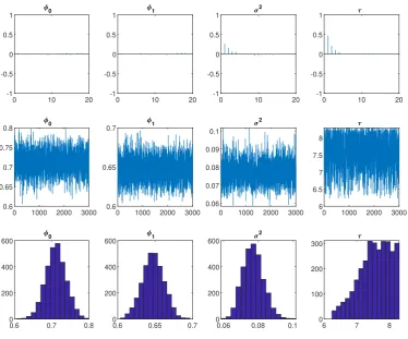
According to the DIC results, the best model is the N B-IN SV, as it has the lowest DIC value (5835.9655). Therefore, we retain theN B-IN SV model in our analysis and report the posterior means and posterior standard deviations (Std) of its parameters in Table 5. For comparison purposes, Table 6 reports the same information concerning the P-IN SV parameters.

All the parameters are statistically significant in both models. In Figure 2, the posterior paths (middle panel) are stable and the posterior autocorrelations (top panel) decay rapidly, suggesting that the proposed MCMC algorithmic scheme for theN B-IN SV model is efficient. This is also confirmed by the reported measures of mixing and convergence (RN I,N SE,CD) in Table 5.

Furthermore, from the posterior histograms (middle panel of Figure 2) of the N B-IN SV param-eters, we observe that φb1 lies in the stability domain, defined by expression (7), while τbis far away

from zero, thus removing any doubt about the validity of the Poisson hypothesis.

Using expressions (14) and (19), the estimates of the mean E(Yt) and variance var(Yt) for the

N B-IN SV model are, respectively, 8.0199 and 26.8621. These values are very close to the sample mean and sample variance of the series. This shows that the estimated model allows a good (two first) moment adjustments. For theP-IN SV case, we haveEb(Yt) = 9.1022 andvard(Yt)= 20.3349.

To examine the adequacy of the N B-IN SV model, we focused on its residuals, which are of two types. First, the Pearson conditional mean residual (_bǫt)1≤t≤n (Y-residuals in short) is defined by

bǫt= q Yt−λbt

b

λt(1+1_bτbλt)

, 1≤t≤n,

where bλt is the BGG estimate of λt, and bλt

1 +_τ1_bbλt

is the estimated conditional variance of the model. Second, the residuals (_bet)1≤t≤n (henceforth e-residuals) of the log-intensity equation are

b

et=σb−1

logλbt

−φb0−φb1log

b

λt−1

, 1_≤t_≤n,

whereφb0,φb1 and bσ2 are the BGGestimates of φ0, φ1 and σ2, respectively.

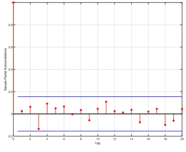
are uncorrelated, and according to Figures 3c (QQ plot) and 3d (kernel density), the normality as-sumption is acceptable. The autocorrelations of the squared and absolute e-residuals have the form of a white noise, which reinforces the independence assumption on the e-innovations; see Figure 4.

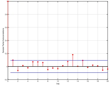
Concerning the analysis ofY-residuals, it can be seen from the simple and partial autocorrelation functions (Figures 5a and 5b, respectively) that there is no significant evidence of correlation within the residuals. However, a visual inspection of Figures 5c (QQ-plot) and 5d (kernel density) reveals that the normality assumption of the residuals is not tenable. It is natural theY-residuals to not have a Gaussian shape because they are residuals from a discrete distribution.

To have a more meaningful conclusion about theBGGfitting we analysed the randomized quantile residuals, defined by Dunn and Smyth (1996) and used e.g. by Benjamin et al., (2003), Zhu (2011) and Aknouche et al., (2018). The randomized quantile residuals are especially useful to achieve continuous residuals, when the series is discrete, as in our case. In the N B-IN SV context, they are given by

b

εt = Φ−1(pt), where Φ−1 is the inverse of the standard normal cumulative distribution and pt is a

random number uniformly chosen in the interval

h

FYt−1;θb

, FYt;θb

i

,

Fx;θbbeing the cumulative function of the negative binomial distribution_{N Bb}τ , bτ b λt+τb

evaluated

atx with parameterθb=φb0,φb1,σb2,bτ

′

.

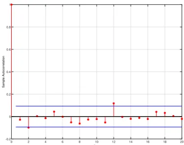
Figure 6 shows the simple and partial autocorrelations of the randomized residuals (panels (a) and (b), respectively), the QQ-plot of these residuals versus the standard normal distribution (panel (c)) and the kernel density (panel (d)). It can be observed that the residuals appear to be roughly a Gaussian white noise as expected, meaning that the distribution of the estimated model fits well to the negative binomial distribution. Similar conclusions can be extracted from the autocorrelation plots of the squared and absolute values of the randomized quantile residuals; see Figure 7.

Finally, Figure 8 displays the evolution of the estimated latent Wct, while Figure 9 shows the

real time path of transaction data along with the estimated conditional mean bλt and the estimated

conditional variance, given by bλt

1 +1_bτbλt

. There is an observed consistent evolution of these two quantities with the evolution of the original series, where the (conditional) overdispersion phenomenon is visually highlighted as well.

In summary, regarding the stability of the N B-IN SV model, the significance of its coefficients, the good mixing of the Gibbs draws and the residual analysis, it can be concluded that the estimated

N B-IN SV model is valid for representing the polio data.

5.2 Polio data

We also applied the proposed Bayesian methodology to the Polio data set, repeating the same empirical analysis that we conducted for the transaction data. The Polio data set, which consists of n = 168 observations, refers to the monthly number of poliomyelitis cases in the United States from January 1971 to December 1983. The time series in question was originally modelled by Zeger (1988) and was later used by many authors (Zeger and Qaqish, 1988; Davis et al., 1999; Benjamin et al., 2003; Davis and Rodriguez-Yam, 2005; Davis and Wu, 2009; Zhu, 2011; Aknouche et al., 2018, among others).

The Polio time series (Figure 10a) with a sample mean of 1.3333 and a sample variance of 3.5050 is clearly overdispersed. The histogram of this data set is given in Figure 10b.

Polio data, which was estimated using the Poisson quasi-maximum likelihood estimation method (P

-QM LE), getting

Xt/Ft−1 ∼ N B

b

τ , τb b τ+bλI

t

, τ_b= 2.6023

( b

λI_t = 0.5808 + 0.1986Yt−1+ 0.7445bλIt−1, 2≤t≤168 b

λI₁ =Y = 1.3333

The prior distributions ofφ,σ2 and τ are given, respectively, by

φ∼N (0.27,0.60)′, diag(0.001,0.001), 5×_σ02.2 ∼χ52, τ ∼ G(0.1,5).

In Table 7, the model comparison results, based on the DIC criterion (Spiegelhalter et al, 2002) show that theN B-IN SV is preferred to theP-IN SV. The estimation results for theN B-IN SV and

P-IN SV models appear in Tables 8 and 9, respectively.

All the parameters are significant in both models. Comparing the two data sets, we notice that the estimated persistence, captured by φ1, is smaller in the Polio data than in the transaction data

for theN B-IN SV model. Furthermore, from the reportedRN I,N SE and CD values (Table 8), as well as the plotted posterior paths and posterior autocorrelations (Figure 11), there are no mixing or convergence problems with the generated Markov chains of the posterior sampler for the dominant model.

Using expressions (14) and (19) of the main paper, the estimates of the mean E(Yt) and variance

var(Yt) for theN B-IN SV model are, respectively, 1.4008 and 3.4966. These values are closer to the

sample mean and sample variance than the corresponding estimated values obtained by Zhu (2011) and Aknouche et al., (2018). This shows that the N B-IN SV model allows for a good (two first) moment adjustments. For theP-IN SV case, Eb(Yt) = 1.6690 andvard(Yt) = 2.4475.

Thee-residual analysis in Figure 12 reveals uncorrelatedness (see also Figure 13) and non-normality. The non-normality is perhaps due to the small sample of the series or to lack of covariates (seasonal effects, etc), as suggested by Zegger (1998) and Davis and Rodriguez-Yam (2005). From theY-residual analysis (Figure 14) and the randomized quantile residual analysis (Figures 15 and 16), the residuals are uncorrelated and resemble a Gaussian white noise process.

In addition, Figure 17 displays the path of the estimated latent Wct variable. Figure 18 confirms

that the data in question suffer for conditional overdispersion.

6

Conclusions

We proposed an integer-valued stochastic volatility (IN SV) model that parallels the stochastic volatil-ity model for real-valued time series. The proposed specification is a discrete-valued parameter-driven model, depending on a latent time-varying intensity parameter, the logarithm of which follows a drifted first-order autoregression. We focused on a rich class of Poisson mixture distributions that form a particular IN SV-type model, the mixed PoissonIN SV model.

innovations, simplifying the study of its probabilistic properties. The second one, which is statistical, allows us to use the scale mixture representation of the conditional distribution of the model, a fact that simplifies the stability of MCMC computation, in particular in the presence of highly volatile (or overdispersed) series.

Under the Gaussianity assumption for the innovation of the log-intensity equation, we considered the Bayesian Griddy-Gibbs sampler in order to estimate the parameters of the mixed PoissonIN SV

model for two particular conditional distributions; the Poisson and the negative binomial. In the negative binomial case we developed two estimation approaches. The first one is based on the direct representation of the negative binomial distribution, while the second one is an improved estimation method, based on the scale mixture representation of the negative binomial distribution. The pro-posed Bayesian methodology is not model-dependent and may be adapted to other important discrete distributions.

0 50 100 150 200 250 300 350 400 450 Time 0 5 10 15 20 25 30 35

Number of transactions

(a) Time series.

0 5 10 15 20 25 30 35 0 20 40 60 80 100 120 140 (b) Histogram.

Figure 1: Transactions per minute for the Ericsson B stock on July 05, 2002.

-1 -0.5 0 0.5 1 0

0 10 20

0 1000 2000 3000 0.6 0.65 0.7 0.75 0.8 0

0.6 0.7 0.8 0 200 400 600 0 -1 -0.5 0 0.5 1 1

0 10 20

0 1000 2000 3000 0.6

0.65

0.7 1

0.6 0.65 0.7 0 200 400 600 1 -1 -0.5 0 0.5 1 2

0 10 20

0 1000 2000 3000 0.06 0.07 0.08 0.09 0.1 2

0.06 0.08 0.1 0 200 400 600 2 -1 -0.5 0 0.5 1

0 10 20

0 1000 2000 3000 6 6.5 7 7.5 8

6 7 8

0 100 200 300

0 2 4 6 8 10 12 14 16 18 20

Lag

-0.2 0 0.2 0.4 0.6 0.8 1

Sample Autocorrelation

(a) Sample autocorrelations of thee-residuals.

0 2 4 6 8 10 12 14 16 18 20

Lag

-0.2 0 0.2 0.4 0.6 0.8 1

Sample Partial Autocorrelations

(b) Partial autocorrelations of thee-residuals.

-4 -3 -2 -1 0 1 2 3 4

Standard Normal Quantiles

-5 -4 -3 -2 -1 0 1 2 3 4

Quantiles of Input Sample

(c) QQ-plot of thee-residuals versus the standard normal

distribution.

-5 -4 -3 -2 -1 0 1 2 3 4 0

0.05 0.1 0.15 0.2 0.25 0.3 0.35 0.4 0.45 0.5

(d) Kernel density of thee-residuals.

0 2 4 6 8 10 12 14 16 18 20

Lag

-0.2 0 0.2 0.4 0.6 0.8 1

Sample Autocorrelation

(a) Sample autocorrelations of the squarede-residuals.

0 2 4 6 8 10 12 14 16 18 20

Lag

-0.2 0 0.2 0.4 0.6 0.8 1

Sample Partial Autocorrelations

(b) Partial autocorrelations of the squarede-residuals.

0 2 4 6 8 10 12 14 16 18 20

Lag

-0.2 0 0.2 0.4 0.6 0.8 1

Sample Autocorrelation

(c) Sample autocorrelations of the absolutee-residuals.

0 2 4 6 8 10 12 14 16 18 20

Lag

-0.2 0 0.2 0.4 0.6 0.8 1

Sample Partial Autocorrelations

(d) Partial autocorrelations of the absolutee-residuals.

Figure 4: Empirical results (Transaction data). Squared and absolute e-residual analysis for the

0 2 4 6 8 10 12 14 16 18 20

Lag

-0.4 -0.2 0 0.2 0.4 0.6 0.8 1

Sample Autocorrelation

(a) Sample autocorrelations of the Pearson residuals.

0 2 4 6 8 10 12 14 16 18 20

Lag

-0.4 -0.2 0 0.2 0.4 0.6 0.8 1

Sample Partial Autocorrelations

(b) Partial autocorrelations of the Pearson residuals.

-4 -3 -2 -1 0 1 2 3 4

Standard Normal Quantiles

-3 -2 -1 0 1 2 3 4 5 6 7

Quantiles of Input Sample

(c) QQ-plot of the Pearson residuals versus the standard normal distribution.

-4 -2 0 2 4 6 8

0 0.05 0.1 0.15 0.2 0.25 0.3 0.35

(d) Kernel density of the Pearson residuals.

0 2 4 6 8 10 12 14 16 18 20

Lag

-0.4 -0.2 0 0.2 0.4 0.6 0.8 1

Sample Autocorrelation

(a) Sample autocorrelations of the randomized quantile residuals.

0 2 4 6 8 10 12 14 16 18 20

Lag

-0.4 -0.2 0 0.2 0.4 0.6 0.8 1

Sample Partial Autocorrelations

(b) Partial autocorrelations of the randomized quantile residuals.

-4 -3 -2 -1 0 1 2 3 4

Standard Normal Quantiles

-4 -3 -2 -1 0 1 2 3 4 5 6

Quantiles of Input Sample

(c) QQ-plot of the randomized quantile residuals versus the standard normal distribution.

-6 -4 -2 0 2 4 6 8

0 0.05 0.1 0.15 0.2 0.25 0.3

(d) Density of the randomized quantile residuals.

Figure 6: Empirical results (Transaction data). Randomized quantile residual analysis for the N B

0 2 4 6 8 10 12 14 16 18 20

Lag

-0.2 0 0.2 0.4 0.6 0.8 1

Sample Autocorrelation

(a) Sample autocorrelations of the squared randomized quantile residuals.

0 2 4 6 8 10 12 14 16 18 20

Lag

-0.2 0 0.2 0.4 0.6 0.8 1

Sample Partial Autocorrelations

(b) Partial autocorrelations of the squared randomized quantile residuals.

0 2 4 6 8 10 12 14 16 18 20

Lag

-0.2 0 0.2 0.4 0.6 0.8 1

Sample Autocorrelation

(c) Sample autocorrelations of the absolute randomized quantile residuals.

0 2 4 6 8 10 12 14 16 18 20

Lag

-0.2 0 0.2 0.4 0.6 0.8 1

Sample Partial Autocorrelations

(d) Partial autocorrelations of the absolute randomized quantile residuals.

Figure 7: Empirical results (Transaction data). Squared and absolute randomized quantile residual analysis for the N B-IN SV model.

0 50 100 150 200 250 300 350 400 450

Time

9.77 9.78 9.79 9.8 9.81 9.82 9.83 9.84

Figure 8: Empirical results (Transaction data). Estimated latent seriesWctfor theN B

-IN SV model.

0 50 100 150 200 250 300 350 400 450

Time

0 10 20 30 40 50 60 70

Transaction series

Estimated intensity Estimated cond. variance

Figure 9: Empirical results (Transaction data). Real series and estimated intensities (conditional mean and variance) for the N B

1970 1971 1972 1973 1974 1975 1976 1977 1978 1979 1980 1981 1982 1983 Year 0 2 4 6 8 10 12 14 Count

(a) Time series.

0 2 4 6 8 10 12 14

0 20 40 60 80 100 120 (b) Histogram.

Figure 10: Monthly number of poliomyelitis cases in the United States from 1970 to 1983.

-1 -0.5 0 0.5 1 0

0 5 10 15 20

0 1000 2000 3000 0 0.05 0.1 0.15 0.2 0

0 0.05 0.1 0.15 0.2 0 200 400 600 0 -1 -0.5 0 0.5 1 1

0 5 10 15 20

0 1000 2000 3000 0.4 0.45 0.5 0.55 0.6 1

0.4 0.45 0.5 0.55 0.6 0 200 400 600 1 -1 -0.5 0 0.5 1 2

0 5 10 15 20

0 1000 2000 3000 0.1

0.15 0.2 0.25

2

0.1 0.15 0.2 0.25 0 200 400 600 2 -1 -0.5 0 0.5 1

0 5 10 15 20

0 1000 2000 3000 0.5

1 1.5 2

2.5

0.5 1 1.5 2 2.5 0

200 400

600

0 2 4 6 8 10 12 14 16 18 20

Lag

-0.2 0 0.2 0.4 0.6 0.8 1

Sample Autocorrelation

(a) Sample autocorrelations of thee-residuals.

0 2 4 6 8 10 12 14 16 18 20

Lag

-0.2 0 0.2 0.4 0.6 0.8 1

Sample Partial Autocorrelations

(b) Partial autocorrelations of thee-residuals.

-3 -2 -1 0 1 2 3

Standard Normal Quantiles

-4 -3 -2 -1 0 1 2 3

Quantiles of Input Sample

(c) QQ-plot of thee-residuals versus the standard normal

distribution.

-3 -2 -1 0 1 2 3 4

0 0.05 0.1 0.15 0.2 0.25 0.3 0.35 0.4

(d) Kernel density of thee-residuals.