Optimal Fiscal Policy Instrument under Different Shocks

ISSN Online: 2162-2086 ISSN Print: 2162-2078

DOI: 10.4236/tel.2017.76115 Oct. 16, 2017 1702 Theoretical Economics Letters

Optimal Fiscal Policy Instrument under

Different Shocks

Shuguang Xing

School of Economics, Peking University, Beijing, China

Abstract

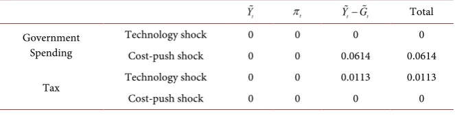
This paper constructs a New Keynesian model to study optimal tax and gov-ernment spending rules and compares their welfare. The output gap, inflation and the difference between the output gap and the government spending gap all affect welfare. This paper finds that the optimal fiscal policy instruments under technical shock and cost-push shock are government spending and tax, respectively. If the policymaker is only concerned with the output gap and in-flation, the optimal fiscal policy rule and actual social welfare loss will change. However, the optimal fiscal policy instruments under technical shock and cost-push shock are still government spending and tax. This paper also finds that an imperfect financial market affects social welfare but does not change the optimal fiscal policy instrument under different shocks.

Keywords

Social Welfare, Tax, Government Spending

1. Introduction

After the financial crisis broke out in 2008, the world economy sank into reces-sion and many countries adopted proactive fiscal policies to stimulate the economy. Between increasing government spending and cutting taxes, which is more effective? Many scholars establish DSGE models to compare the effects of tax and government spending. Denes and Eggertsson [1] and Eggertsson [2] argue that when the nominal short-term interest rate is zero, a tax cut leads to deflation, which in turn increases recession, while increasing government spending is more effective. Erceg and Linde [3] study the effect of increasing taxes and decreasing government spending on output to meet fiscal constraints in a monetary union. Given the limited scope for monetary accommodation, raising taxes has a smaller adverse effect on output compared to cutting government spending in the short How to cite this paper: Xing, S.G. (2017)

Optimal Fiscal Policy Instrument under Different Shocks. Theoretical Economics Letters, 7, 1702-1712.

https://doi.org/10.4236/tel.2017.76115

Received: September 4, 2017 Accepted: October 13, 2017 Published: October 16, 2017

Copyright © 2017 by author and Scientific Research Publishing Inc. This work is licensed under the Creative Commons Attribution International License (CC BY 4.0).

http://creativecommons.org/licenses/by/4.0/

DOI: 10.4236/tel.2017.76115 1703 Theoretical Economics Letters term but has a bigger adverse effect in the long term. If the interest rate is close to zero, the impact of cutting government spending on output increases.

Most related empirical studies use SVAR models. Blanchard and Perotti [4] find increasing government spending has a positive effect on output, and creasing taxes has a negative effect, and they both have a negative effect on in-vestment spending. Mountford and Uhlig [5] and Caldara and Kamps [6] find that the multiplier of tax cuts is greater than that of increasing government spending. Batini et al. [7] find that in order to meet fiscal constraints, increasing taxes has a less adverse effect on output than cutting government spending. In addition, Arin et al. [8], using Bayesian model averaging, find that productive public spending has a positive effect on output, while top corporate tax rates have a negative effect, and fiscal variables with no robust effect on output in-clude top income tax rates, government consumption, and distortionary taxes.

The studies are only concerned with the effect of fiscal policy on output. However, what affects social welfare includes not only output but also inflation and other things. What is more, they ignore the different effects of fiscal policy under different shocks. This paper constructs a simple New Keynesian model to study optimal fiscal instruments under different shocks. In contrast with Wood-ford [9], the welfare loss function in this paper includes not only the output gap and inflation but also the difference between the output gap and the government spending gap. The optimal tax and government spending rules are given and their welfare losses are compared. Tax can stabilize cost-push shock, but not technology shock, while government spending can stabilize technology shock, but not cost-push shock. This means that the optimal fiscal policy instrument under technical shock is government spending, and the optimal fiscal policy in-strument under cost-push shock is tax.

If a policymaker is only concerned with the output gap and inflation, tax and government spending will eliminate the effects of cost-push shock and technol-ogy shock on marginal costs and then further eliminate the output gap and in-flation. However, the actual welfare loss increases when using tax (government spending) to stabilize technology (cost-push) shock.

Finally, this paper assumes that households cannot access the financial mar-ket. In this case, the optimal fiscal policy instruments under technical shock and cost-push shock are still the government spending and tax respectively, and both they can achieve the effective allocation.

This paper is organized as follows. Section 2 constructs a New Keynesian model. Section 3 log-linearizes the welfare function and constraint conditions. Section 4 considers the optimal tax rule and the optimal government spending rule and compares their welfare. Section 5 analyzes the impact of imperfect fi-nancial markets on fiscal rules and social welfare. Section 6 is the conclusion.

2. Model

dis-DOI: 10.4236/tel.2017.76115 1704 Theoretical Economics Letters tributed in the [0, 1] interval. Each household is both a consumer and a produc-er. The product market is monopoly competition. Firms are owned by house-holds. In addition, households have access to perfect financial markets.

Each household has the same preference. Suppose that the elasticity of the in-tertemporal substitution of consumption and the wage elasticity of labor supply are both 1. The representative household maximizes the utility function:

(

)

0

ln 1 ln

t

t t t

t

E∞

β χ

C

χ

G L

=

+ − −

 

 

∑

(1) where E is the expectation, β is the discount factor, Ct is the consumption index,

Lt is the labor time, χ is the ratio of consumption to government expenditure in utility. This form of utility function is easy for us to derive the second-order welfare loss function.

The budget constraint of household is:

, 1 1

t t t t t t t t t t t t

PC E Q D+ + + ≤W L D+ + Π − ΓP

₍₂₎

where Pt is the price level, Dt+1 is the nominal return on the asset held by the household in period t + 1, Qt,t+1 is the random discount factor, Wt is the nominal wage, Πt is the firm’s profit, Γt is the lump tax. Household consumption Ct is a set of products with differentiated products, Ct ₀1C it

( )

( 1) di ( 1)

θ θ

θ− θ −

 

≡ _

∫

_ ,

defined by Dixit and Stiglitz [10], and θ >1 _{is the elasticity of the product}

substitution.

Under the budget constraint and transversal condition _Tlim_→∞E Q Dt

(

tT T

)

=0,

the optimal labor supply equation can be obtained by maximizing the utility function:

1 1 t

t t

W P C

χ =

(3) Equation (3) shows that the positive marginal utility of increasing labor supply is just equal to its negative marginal utility. We can also get the Euler eq-uation:

1 1

1 1 t

t t

t t t

P

E R

C

β

C P+ +

 

= _{ }

 

(4)

where Rt

(

E Qt t t, 1

)

1 − +

≡ _{. Equation (4) reflects the optimal consumption path.}

Consistent with the traditional New Keynesian model, capital is not consi-dered here. There is a continuum of monopoly firms represented by the interval [0, 1]. The product function is:

( )

( )

t t t

Y i =A L i

(5) where Y it

( )

is the product of firm i in period t, L it

( )

is the labor demand,

t

A is the level of technology, assumed to be common to all firms and to evolve exogenously over time. Following Calvo [11], the firm resets price P it

( )

with a

DOI: 10.4236/tel.2017.76115 1705 Theoretical Economics Letters

(

) ( ) ( ) (

)

( )

, 1 1

T t

t t T T t T T T

T t

E ∞

α

−Q

τ

P i Y i

η

W L i = − − −    

∑

(6) where τt is the sales tax rate, η is the government subsidies at steady state to

eliminate the monopoly distortion. The first-order condition for this optimal problem is:

(

) ( )

(

)

(

( )

)

1

( )

, 1 t 1 0

T t T

t t T T T T t T

T t T T

P i Y

E Q Y W P i P

P A

θ

θ θ

α τ µ η

− ∞ _{− −} − =  _{ }   − _{ } − − =      

∑

(7) where 1 θ µ θ ≡

− , denotes price markup. Yt is the output, defined as

( )

( ) ( )1

1 1

0 d

t t

Y _ Y i θ− θ i_θ θ−

≡ 

∫

 .

Calvo pricing means the price follows the rule:

(

) ( )

1 1 1( )

1

1 1

t t t

P _αP−θ _α P i −θ −θ −

 

=_ + − _

(8)

3. Log-Linearization

Log-linearization first requires determining the steady-state value of each varia-ble. In the steady state, there are no exogenous shocks. Assume A=1_{, so} Y L= _.

Social planner maximizes the welfare function

χ

lnC+ −

(

1

χ

)

lnG L− _{, under}

resource constraint Y C G= + _{. The optimal steady state values are} Y=1_,

C=

χ

_, G= −1

χ

_{. Social planner at the steady state eliminates monopoly}

distor-tion through subsidy.

When the price is flexible, Lt =1, Yt=At, Ct =χAt, Gt= −

(

1

χ

)

At. If there

is no monopoly distortion under flexible price, a decentralized economy can achieve the effective allocation.

Define Xˆ_t≡log

(

X X_t

)

, Xˆt denotes the log-deviation of Xt from its steady state X under sticky price; Define ˆn log

(

n

)

t t

X ≡ X X _, ˆn t

X denotes the log- deviation of Xt from its steady state X under flexible price; Define Xt ≡Xˆt−Xˆtn,

t

X denotes the gap between Xˆt and its natural rate Xˆtn. Then, we have ˆ

ˆn

t t

Y =A , ˆn ˆ

t t

C =A, ˆn ˆ

t t

G =A.

When the price is sticky, the welfare loss function can be obtained by the second-order approximation method of Woodford [10]:

(

)

2

( )

3

2 2 0 0 1 1 2 t

t t t t

t

W E Y Y G tip O

k

θ χ

β π ξ

χ ∞ =  −  = − _ + + − _+ +  

∑

(9) where tip is the terms independent of policy including constants and functions of exogenous shocks, _O

( )

_ξ 3 _{stands for the terms that are of order higher}

than the second, k

(

1

α

)(

1

αβ

)

α

− −

≡ _, Y Y A_t ≡ −ˆ_t ˆ_t, π_{t is inflation. The larger}

the output gap or inflation, the smaller the welfare. 1

(

Y Gt t

)

2

χ

χ

− ₋

reflects the second-order effect of government spending crowding out consumption. When

1

DOI: 10.4236/tel.2017.76115 1706 Theoretical Economics Letters Log-linearizing optimal pricing rule can obtain the New Keynesian Phillips curve:

1

1 1 _{1 ˆ ˆ}

t k Yt Gt t t Et t

χ

π τ µ β π

χ χ θ +

 − 

= _ − + + _+

  (10)

where µˆ_{t denotes the cost-push shock. An increase in output increases labor}

demand and leads to an increase in wage, which in turn increases marginal cost and inflation. The smaller the price stickiness, the larger k, then the higher the inflation caused by the increase in output. Increasing the tax rate raises the mar-ginal cost and increases inflation. Given the output, government spending will crowd out consumption. According to Equation (3), the real wage will fall, which will reduce inflation. When firms expect an increase in inflation, they raise prices, which in turn leads to inflation.

Log-linearizing Euler equation can obtain the New Keynesian IS curve:

(

)

(

)

1 1 ˆ 1 1 1

t t t t t t t t t t

Y E Y = ₊ −

χ

i E−

π

₊ − − ∆i E A₊ − −

χ

E G∆₊

(11) where i≡1β−1_{. When the interest rate rises, current consumption declines,}

resulting in a decline in output. Meanwhile, increasing government spending will lead to higher output.

4. Optimal Fiscal Policy

If both tax and government spending can be used, efficient allocation will be achieved. Then, Yt=0, π =t 0, Gt=0, τˆt = −θµˆt, i i E At= + ∆t ˆt+1. The follow-ing analyzes the optimal tax and government spendfollow-ing rules.

4.1. Optimal Tax Rule

Under the constraints of Equations ((10) and (11)), the central bank and fiscal authority choose

{

Yt, , ,

π τ

t i ˆt

}

to the maximize welfare loss function Equation

(9). The optimal tax and monetary rules are:

(

₁

)

ˆ

t t

Y = − −

χ

A

(12)

0 t

π = ₍₁₃₎

ˆ_t ˆ_t

τ = −θµ ₍₁₄₎

1

ˆ

t t t

i i E A= + ∆ + ₍₁₅₎ From Equation (14), we know that tax does not change under technology shock, but decreases with the increase of cost-push shock to completely eliminate the impact of cost-push shock on marginal cost. When there is a technology shock, the tax rule is τ =ˆ 0t , and the interest rate rule is i i E At= + ∆t ˆt+1. Then,

0 t

π = _, Yt= − −

(

1

χ

)

Aˆt. Because the fiscal instrument is tax, so Gˆ 0t = , then ˆ

t t

G = −A. So Yt≠0, Y Gt− t≠0, that means tax cannot stabilize the technology

shock. When there is a cost-push shock, the tax rule is τˆ_t = −θµˆ_{t, and the interest}

rate rule is i it = . Then, Yt=0, π =t 0, Gt =0, that means tax can stabilize the

DOI: 10.4236/tel.2017.76115 1707 Theoretical Economics Letters

4.2. Optimal Government Spending Rule

Under the constraints of Equations ((10) and (11)), the central bank and fiscal authority choose

{

Yt, , ,

π

t ti Gt

}

to the maximize welfare loss function. The

op-timal government spending and monetary rules are:

1 1 ˆ

t t t t t

Y =

ϖβ

E Y+ +

ϖ

Y− −

ϖθ µ

k ₍₁₆₎

1

t Yt

π θ

= − ∆

(17)

0 t

G = ₍₁₈₎

1 ˆ 1

1

t t t t t

i i θ Eπ E A

χ + +

 

= + −_{ } + ∆

  (19) where

(

)

1 k

χ ϖ

β χ θ

≡

+ + . Under a technology shock, government spending can achieve the effective allocation, that means Yt=0, π =t 0, Gt=0. The interest

rate rule is i i E At= + ∆t ˆt+1. Under a cost-push shock, Yt and πt are not zero,

the effective allocation cannot be achieved. Meanwhile, G Gˆt= t=0,

1

1

t t t

i i θ Eπ

χ +

  = + −_{ }

  .

4.3. Simulation

To more intuitively compare the welfare losses of tax and government spending, this paper will conduct simulations. All the parameter values are commonly used in the literature. The discount rate β is 0.99, the elasticity of product substitution θ is 11, the price stickiness index α is 0.8, the share of consumption in output in steady state χ is 0.7 in the steady state, and the tax rate in the steady state τ is 0.3. The shocks are AR (1) processes with autoregressive coefficient 0.9 and innova-tion variance 0.01. The simulainnova-tion software is Dynare 4.4.3 running with MATLAB 2013.

According to Woodford [9] and Gali [12], welfare loss can be expressed as:

( )

( )

(

)

1 _{var var} 1 _var

2 t t t t

W Y Y G

k

θ _π χ

χ

 − 

= _ + + − _

  (20)

where var(X) denotes the variance of X.

Table 1 shows the welfare losses under technology shock and cost-push shock. Consistent with the above analysis, government spending can fully stabilize technology shock to achieve effective allocation, and the welfare loss is zero. If tax is used to stabilize technology shock, the welfare loss is 0.0079. That means wel-fare loss accounts for 0.79% of output in the steady state. The output gap, infla-tion, and the difference between the output gap and the government spending gap cause welfare loss by 0.0024, 0, and 0.0055, respectively. This case is the same as in the absence of fiscal policy, and tax under technology shock is superfluous.

DOI: 10.4236/tel.2017.76115 1708 Theoretical Economics Letters which accounts for 1.61% of output in steady-state. The output gap, inflation, and the difference between the output gap and the government spending gap cause welfare loss by 0.0102, 0.0015, and 0.0044, respectively. That is, the same as in the absence of tax under technology shock.

4.4. Alternative Welfare Objective

Equation (9) shows that welfare loss is caused by Yt, πt and Y Gt− t three

parts. What occurs if a policymaker is only concerned about the output gap and inflation? The welfare loss function in this case is:

( )

3

2 2

0 0

1 2

t

t t

t

W E Y tip O

k

θ

β

π

ξ

∞

=

 

= − _ + _+ +

 

∑

(21) The central bank and fiscal authority choose

{

Yt, , ,

π τ

t i ˆt

}

and

{

Yt, , ,

π

t ti Gt

}

to maximize welfare loss function (21) under the constraints of Equations ((10) and (11)). The optimal path of each variable under tax policy is: Yt=0, π =t 0,

(

1

)

_ˆ

ˆ_t χ θ A_t ˆ_t

τ θµ

χ −

= − − _, i i E A_t= + ∆_t ˆ_t+₁. In this case, tax decrease with the in-creasing of technology shock and cost-push shock to offset their effects on the marginal cost. The optimal path of each variable under government spending policy is: Yt =0, π =t 0, Gt ₁ ˆt

χ

µ

χ

= −

_, ˆ _{1 ˆ 1}

t t t t t

i i E A= + ∆ + − ∆E

µ

+ . Government spending can eliminate the output gap and inflation. [image:7.595.207.540.464.585.2]

As shown in Table 2, although the output gap and inflation both are zero, the real welfare loss function expressed as Equation (20) is worse when using govern-ment spending to stabilize cost-push shock or using tax to stabilize technology

Table 1. Welfare Losses.

t

Y π_t Y G_t−_{t Total} Government

Spending

Technology shock 0 0 0 0 Cost-push shock 0.0102 0.0015 0.0044 0.0161

Tax Technology shock 0.0024 0 0.0055 0.0079 Cost-push shock 0 0 0 0

No Fiscal Policy Technology shock 0.0024 0 0.0055 0.0079 Cost-push shock 0.0102 0.0015 0.0044 0.0161

Notes: The values in the third, fourth and fifth column are welfare losses caused by Yt, πt, and Y Gt−t,

respectively. The values in the sixth column are the total Welfare losses. The same below.

Table 2. Welfare Losses Under Alternative Welfare Objective.

t

Y π_t Y G_t− _t Total Government

Spending

Technology shock 0 0 0 0 Cost-push shock 0 0 0.0614 0.0614

[image:7.595.208.540.642.727.2]

DOI: 10.4236/tel.2017.76115 1709 Theoretical Economics Letters shock. However, the optimal fiscal policy instruments for technology shocks and cost-push shocks are still government spending and tax, respectively.

5. Imperfect Financial Market

As per Gali et al. [13], this paper will analyze households without access to the financial market. The households cannot use bonds to smooth consumption as before. The budget constraint of households is:

t t t t

PC W L= ₍₂₂₎

From Equations ((3) and (22)), we can get:

t

L =χ ₍₂₃₎

Equation (23) means if households cannot access the financial market, labor supply is constant. We get:

ˆ

ˆ _{, 0}

t t t

Y A Y= = ₍₂₄₎

The welfare loss function under an imperfect financial market is:

( )

3

2 2

0 0

1 1

2

t

t t

t

W E G tip O

k

θ χ

β π ξ

χ

∞

=

 − 

= − _ + _+ +

 

∑

(25) The New Keynesian Phillips curve is:

1

1 _{1 ˆ ˆ}

t k Gt t t Et t

χ

π τ µ β π

χ θ +

 − 

= _− + + _+

  (26)

The central bank and the fiscal authority choose

{

π τ

t,ˆt

}

and

{

π

t,Gt

}

to

the maximize welfare loss function (25) under the constraint of (26). The optim-al path of each variable under the optimoptim-al tax policy is: Yt=0, π =t 0,

(

1

)

_ˆ

ˆ_t χ θ A_t ˆ_t

τ θµ

χ −

= − − _, G_t = −Aˆ_{t. As in the perfect financial market, tax can} stabilize cost-push shock, but not technology shock.

When the fiscal instrument is government spending, the optimal government spending rule is:

1 1 ˆ

t t t t t

G =

ωβ

E G+ +

ω

G− +

ωθ µ

k

₍₂₇₎

where

(

)

(

)

1 k 1

χ ω

χ θ β χ

≡

− + + .

The inflation target is:

1

t Gt

π θ

= ∆

(28) From Equations ((27) and (28)), we can get Gt =0, π =t 0, under technology

shock, but G_t≠0_, π ≠t 0, under technology shock. So as in the perfect

finan-cial market, government spending can stabilize technology shock, but not cost-push shock.

[image:9.595.208.541.90.175.2]

DOI: 10.4236/tel.2017.76115 1710 Theoretical Economics Letters

Table 3. Welfare Losses Under the Imperfect Financial Market.

t

Y π_t Y Gt− t Total

Government Spending

Technology shock 0 0 0 0 Cost-push shock 0 0.0077 0.0382 0.0459

Tax Technology shock 0 0 0.0113 0.0113 Cost-push shock 0 0 0 0

market, the optimal fiscal policy instruments under technology shock and cost-push shock are government spending and taxation. What is more, govern-ment spending (tax) harms social welfare under cost-push (technology) shock.

6. Conclusions

Many studies compare the difference between the tax multiplier and government spending multiplier, but they only focus on the effect of fiscal policy on output, not on social welfare. In addition, these studies also ignore that the effects of fis-cal policy are different under different shocks. In this paper, a simple New Key-nesian model is established to study the optimal tax and government spending rules and compares their welfare difference. This paper finds that the optimal fiscal policy instruments under technical shock and cost-push shock are gov-ernment spending and tax, respectively. The factors affecting social welfare in-clude the output gap, inflation, and the difference between the output gap and the government spending gap. If the policymaker is only concerned with the output gap and inflation, the actual social welfare loss will change. However, the optimal fiscal policy instruments under technical shock and cost-push shock are still government spending and tax, respectively. Finally, this paper assumes that households cannot access the financial market. In this case, the optimal fiscal policy instrument under different shocks does not change.

There are rooms of improvement in this paper. In order to simplify the model, this paper sets the relative risk aversion coefficient to one, and a general utility function can be set up in the future. In addition, this paper does not consider fiscal budget, and government sector can be introduced into the model. Finally, interest rate in many developed countries approaches to zero, and this means fiscal policy is more important, and we can study the optimal fiscal instrument in this case.

References

[1] Denes, M. and Eggertsson, G.B. (2009) A Bayesian Approach to Estimating Tax and Spending Multipliers. FRB of New York Staff Report 403.

https://doi.org/10.2139/ssrn.1504845

[2] Eggertsson, G.B. (2011) What Fiscal Policy Is Effective at Zero Interest Rates? NBER Macroeconomics Annual, 25, 59-112. https://doi.org/10.1086/657529

DOI: 10.4236/tel.2017.76115 1711 Theoretical Economics Letters

https://doi.org/10.1016/j.jedc.2012.09.012

[4] Blanchard, O. and Perotti, R. (2002) An Empirical Characterization of the Dynamic Effects of Changes in Government Spending and Taxes on Output. The Quarterly Journal of Economics, 117, 1329-1368.

https://doi.org/10.1162/003355302320935043

[5] Mountford, A. and Uhlig, H. (2009) What Are the Effects of Fiscal Policy Shocks? Journal of Applied Econometrics, 24, 960-992. https://doi.org/10.1002/jae.1079

http://onlinelibrary.wiley.com/doi/10.1002/jae.1079/full

[6] Caldara, D. and Kamps, C. (2012) The Analytics of SVARs: A Unified Framework to Measure Fiscal Multipliers. Board of Governors of the Federal Reserve System WP.

[7] Batini, N., Callegari, G. and Melina, G. (2012) Successful Austerity in the United States, Europe and Japan. IMF Working Paper WP/12/190.

[8] Arin, K.P., Braunfels, E. and Doppelhofer, G. (2015) Taxes, Spending and Economic Growth: A Bayesian Model Averaging Approach. Cesifo WP.

[9] Woodford, M. (2003) Interest and Prices: Foundations of a Theory of Monetary Policy. Princeton University Press, Princeton.

[10] Dixit, A. and Stiglitz, J. (1977) Monopolistic Competition and Optimum Product Diversity. American Economic Review, 67, 297-308.

[11] Calvo, G. (1983) Staggered Prices in a Utility Maximizing Framework. Journal of Monetary Economics, 12, 383-395. https://doi.org/10.1016/0304-3932(83)90060-0 [12] Gali, J. (2008) Monetary Policy, Inflation, and the Business Cycle: An Introduction

to the New Keynesian Framework. Princeton University Press, Princeton.

[13] Gali, J., Lopez-Salido, J.D. and Valles, J. (2007) Understanding the Effects of Gov-ernment Spending on Consumption. Journal of the European Economic Associa-tion, 5, 227-270. http://onlinelibrary.wiley.com/doi/10.1162/JEEA.2007.5.1.227/full

DOI: 10.4236/tel.2017.76115 1712 Theoretical Economics Letters

Appendix A: Log-Linearization of Welfare Objective

Taking second-order approximations to the representative household’s utility function, we can get:

(

)

(

) ( )

(

) (

)

( )

(

)

( )

2 2 2 3 2 3 2

ln 1 ln

1 2

1 2

1 ˆ ₁ ˆ ˆ ˆ

2

t t t t

t

t t

t t

t t t t

U C G L

C C

C C G G

C C G

G G _LL L _{tip O}

L G

C G L L L tip O

χ χ

χ

χ χ

χ

ξ

χ χ ξ

= + − − − − − = − + − − − − − − + +   = + − − _ + _+ +   (A.1)

From the firm’s production function, we can get:

t t t t Y L A ∆ = (A.2)

where ₀1 t

( )

d t

t

P i _i

P θ −   ∆ ≡    

∫

, denotes the price dispersion. (A.2) can be log-linearized as:

ˆ

ˆ ˆ ˆ

t t t t

L Y= + ∆ −A

_(A.3) According to (A.3), (A.1) can be rewritten as:

(

)

1

(

)

2

( )

3

ˆ ₁ ˆ ˆ ˆ ˆ ˆ

2

t t t t t t t

U =

χ

C + −

χ

G − ∆ + +_ Y Y A− _+tip O+

ξ

  (A.4)

The market clearing condition is:

t t t

Y C G= + _(A.5)

Above equation can be log-linearized as:

(

)

2

2

1 1 1

ˆ ˆ ˆ ˆ ˆ

2

t t t t t

C =_χY − −_χχG − −_χχ Y G−

(A.6) According to Woodford (2003), we have:

(

)(

)

2

( )

3

0 0

1 ˆ

2 1 1

t t

t t

t t tip O

αθ

β β π ξ

α αβ ∞ ∞ = = ∆ = + + − −

∑

∑

(A.7) According to (A.4), (A.6) and (A.7), social welfare can be rewritten as:

(

)

2 ₂

(

)

2

( )

₃

0 0

1 _{ˆ ˆ} 1 _{ˆ ˆ} 2

t

t t t t t

t

W E Y A Y G tip O

k

θ χ

β π ξ

χ ∞ =  −  = − _ − + + − _+ +  

∑

(A.8) Since the definition ˆ ˆn

t t t

X ≡X −X _{, and} ˆn ˆ

t t

Y ≡A _{, (A.8) can be rewritten as:}

(

)

2

( )

₃

2 2

0 0

1 1

2 t t t t t t

W E Y Y G tip O

k

θ χ

β π ξ