Do Redistributive Policies Affect Economic Growth?

Do Redistributive Policies Affect Economic Growth?

——An Empirical Study based on Canadian data

Zheng Liu

Department of Economics, Concordia University, Montreal, Canada Email: jacquesliu@gmail.com

Received2012

ABSTRACT

To reduce income inequality, redistributive policies are widely adopted by both federal and provincial governments in Canada. Quebec and Canada have a fairer society in OECD countries. However, their economic growth is slower than many other countries. This paper studies how these redistributive policies affect economic growth based on Canadian data for the first time. The growth model is based on standard augmented Solow model and includes several different self-defined policy indexes. Using high quality panel data spanning the period 1982 to 2009 calculated from statistic Canada’s website and Arellano-Bond panel technique, empirical analyses show that redistributive policy is negatively and significantly associated with economic growth. These findings are in accordance with many former literatures and may have important policy significance.

Keywords: Income Inequality and Economic Growth

1.

Introduction

Canada, especially Quebec, is one of the best areas around the world on reducing income inequality. How-ever, there is a debate whether Canadian benefit from a more equal society.

The key of the debate is whether income inequality will affect economic growth, which is a classical eco-nomic question. Since Nobel laureate Simon Kuznets introduced his Kuznet’s curve which shows inequality first rises and later falls with economic growth, many economists have made their contribution on this topic theoretically or empirically. These studies either find a negative or a positive coefficient on inequality. Alesina and Rodrik (1994), Benabou (1996), and William Eas-terly 2006, etc conclude inequality does cause underde-velopment. However, Li and Zou (1998), Kristin Forbers (2000), Mark Patridge (2004), Mark Frank( 2009) and many authors argue that inequality is not harmful for growth. Robert Barro (1999) follows Kuznet’s tradition and concludes that inequality retards growth in poor countries but encourages growth in richer places. Qual (2001) also finds little relationship between inequality and growth.

Why income inequality has negative or positive influ-ence on economic growth? Many theories have been proposed. On negative side, first, credit-market imper-fection models suggest a transfer payment from rich to poor raises the average productivity of investment. In the

presence of asymmetric information and limited access to credit, investments favor people with more assets. Se-condly, high income inequality in a society will often bring social unrest even revolution. Poor people are easy to engage in crime, riots and disruptive activities which are a waste of social resources. Therefore, higher inequa-lity means more social resource waste and lower eco-nomic growth. Thirdly, under Alesina and Rodrik’s polit-ical economy model, a system of majority voting tends to redistributive policies from rich to poor and many public expenditure programs. Poor people will lose interest to work again and rich people will have to prevent this redi-stributive policy through bribery. Often there is no enough investment in the economy and economic growth slows down.

reduce economic growth.

Clearly, no either of above theories can fully explain the effect of income inequality on economic growth. This point accords with the ambiguous empirical findings in many literatures. Level of development, political institu-tions, and many other factors will decide whether it is positive or negative relation between income inequality and economic growth.

This paper will take Canada as an example. Veall (2012) in his most recent paper concludes that the surge in top share incomes in Canada over the last 30 years is clear. At the same time, redistributive policies – namely, mainly taxes and transfers – are widely used by both federal and provincial governments. The effect of redi-stributive policies of Canadian governments on economic growth is studied for the first time (according to our sur-vey) in this paper. Section 2 explains our growth model and dataset. Section 3 estimates this model based on the panel technique developed by Allreno and Bond. Section 4 is some discussion followed by a simple conclusion.

2.

Growth Model and Dataset

This paper estimates growth as a function of redistribu-tive policy index, lagged per capita income, investment share, education, and working population growth rate using a model similar to the augmented Solow model in N.Gregory Mankiw, David Romer and David N. Weil’s (MRW) 1992 paper. Besides using per capita GDP growth rate instead of per capita income as the dependant variable, the only other change from MRW’s original model is the addition of policy index.

The growth model central to this paper is

it 1 i,t 1 2 i,t

3 i,t 4 i,t

5 i,t i,t

GrowthβIncomeβEducation

βInvestmentβPopulation

βRedistributive_Policy u

−

= +

+ +

+ +

(1)

where represents each province in Canada and t represents each time period; is average an-nual growth rate of per capita GDP for province dur-ing period t; is per capita GDP for prov-ince in time period t-1; Unlike MRW’s paper using the percentage of the working-age population that is in sec-ondary school as education index, this paper will use a new education index. In developed country such as Can-ada, there is very little difference on secondary school enrollment rate for each province. Therefore, it is not a good education index again. We decide to use school board expenditure as the new education index in this pa-per because it is easy to acquire long span data.

As in MRW’s paper, this paper uses average share of real investment (including government investment) in

real GDP as investment index and average rate of growth of the working-age population (15-64) as population in-dex. The same as in MRW’s paper, we use n g+ +δ (Assuming gδ+ =0.05 ) to be the population item.

Several redistributive policy indexes are used in this paper. The first one is change of Gini coefficient before and after execution of redistributive policies. Gini coeffi-cient is widely used in many inequality-growth literatures. Traditionally, redistribution could be achieved by many methods like progressive income tax, capital tax, mini-mum wage laws, public expenditure of government and others. Gini coefficient, as a good indicator of income distribution, reflects result of redistributive policies di-rectly, especially the change of Gini coefficient before and after execution of redistributive policies.

When there is no accurate Gini coefficient data availa-ble, which is possible in many developing countries, two other policy indexes are defined based on income distri-bution change. Figure 1 gives an illustration of income distribution change using data from Alberta, Ontario and Quebec in three different periods. Y-axis shows the ratio of change and X-axis shows quintile. The figure clearly shows Quebec has much stronger redistributive policy than Alberta. Based on figure 1, the second and the third policy index are the average slope and the regression slop (from polyfit operation) of the income distribution change line respectively. All three policy indexes are set to be positive.

This paper will use all these different policy indexes and give a comparison. At last, is the error term of the model.

-.5

0

.5

1

1.5

-.5

0

.5

1

1.5

20 40 60 80 100

20 40 60 80 100

QC ON

AB

1981 1995

2006 quntile

Graphs by Province

Figure 1: Illustration of income distribution change

suffi-cient variation in income distribution to produce diffe-rential economic outcomes. Secondly, large factor flows between states should magnify how small disparities in initial conditions affect economic growth. Thirdly, the great homogeneity of state-level data helps mitigate the possible omitted variable bias. Similarly, this paper uses data from 10 provinces from 1982 to 2009 in Canada. All data are from website of Statistics Canada (CANSIM). Clearly, high quality is another important advantage to use data from CANSIM.

3.

Empirical Results

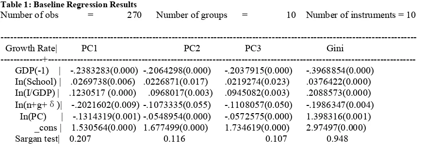
Empirical study of effect of inequality on economic growth often bases on different regression methods. There are either OLS regressions over a cross-section of nations or panel techniques over both periods and geo-graphic regions. Forbes(2000) once pointed out to eva-luate which technique is optimal, there are three factors: (1) the relationship between the region-specific effect and the regressors; (2) the presence of a lagged endo-genous variable; (3) and the potential endogeneity of the other regressors. The same as Forbes, this paper will use Arellano-Bond method to study the income inequali-ty/economic growth effect. Standard panel techniques like fixed effects and random effects have an important problem that there is a lagged endogenous income varia-ble in the growth model. Manuel Arellano and Stephen R.Bond (1991) developed a special panel technique which corrects not only for the bias introduced by the lagged endogenous variable, but also permits a certain degree of endogeneity in the other regressors. This me-thod can eliminate the region-specific effect and then uses all possible lagged values of each of the variables as instruments through first-difference. Table 1 lists the estimation result.

As Table 1 shows, the regression coefficients of all three policy indexes are negative and significant. In all three cases, the higher policy-index means more transfer payment for the poor and higher tax for the rich. This result is consistent with the simple theory model in Li and Zou (1998)’s paper. When public consumption enters utility function, income inequality has a positive relationship with economic growth. In Canada, especially in Quebec, government spends a lot on public services like education, public health, pension plan etc. It is easy for residents to lose incentive to work harder and it is hard for government to find enough capital to invest for economic growth.

Comparing three policy indexes from column 2 to column 4, no much difference is found although PC1 has a better Sargan test result. This shows Gini change is a better policy index compared to others in our regression. This result is also consistent with former panel data

lite-ratures where income inequality has a positive relation-ship with economic growth. As a comparison, column 5 gives the positive regression result on Gini coefficient in our model.

For the other explanatory variables, all the regression coefficients are significant. The coefficients of lagged per capita GDP and population growth rate are negative, and the coefficients of education and investment are pos-itive. These results are consistent with results of aug-mented Solow model and other researchers’ findings. In Allreno-Bond estimation, instruments setup is very important in order to get the ideal result. To improve efficiency of instruments, first is to choose endogenous and exogenous variables. In this paper we choose lagged per capita GDP and investment share to be endogenous and policy index as exogenous variable. Secondly, “sys-tem GMM” is introduced to further improvement instru-ments. The “system GMM” estimator uses the levels equation to obtain a system of two equations: one diffe-renced and one in levels. By adding the second equation additional instruments can be obtained. Third, there is a rule of thumb in Allreno-Bond method which is to keep the number of instruments less than or equal to the num-ber of groups. In this paper, because we have only 10 provinces (groups), we must be very careful on selection of the instruments. Here “collapse” inside gmm() option is used to reduce the number of instruments.

Sensitivity analysis is usually an important step to examine the robustness of baseline regression results. To do sensitivity analysis, more variables are required to be added into the growth model. In this paper, only two more sensitive variables, international trade share and R&D expenditure share over GDP share, are considered. In step 1, both two sensitive variables are included. In step 2 and 3, only one sensitive variable is added each time.

Table 2 shows results of the simple sensitivity analy-sis. When sensitive variables are added, first, better Sar-gan test value shows that instruments setup improves. Secondly, more variables including sensitive variables become insignificant. Thirdly, the regression coefficients of policy index keeps negative and significant. This find-ing seems to confirm that the negative relationship between income inequality and economic growth is robust.

4.

Discussion

It is important to note that there are still several questions for further discussion. These will be explained in this section.

(1) Measurement-error and omitted variable

bias

Table 1: Baseline Regression Results

Number of obs = 270 Number of groups = 10 Number of instruments = 10

--- Growth Rate| PC1 PC2 PC3 Gini

---+--- GDP(-1) | -.2383283(0.000) -.2064298(0.000) -.2037915(0.000) -.3968854(0.000)

In(School) | .0269738(0.006) .0226871(0.017) .0219274(0.023) .0376422(0.000) In(I/GDP) | .1230517 (0.000) .0968017(0.003) .0945082(0.003) .2088573(0.000) In(n+g+δ_{)| -.2021602(0.009) -.1073335(0.055) -.1108057(0.050) -.1986347(0.004)}

In(PC) | -.1314319(0.001) -.0548954(0.000) -.0572575(0.000) 1.398316(0.001) _cons | 1.530564(0.000) 1.677499(0.000) 1.734619(0.000) 2.97497(0.000)

Sargan test| 0.207 0.116 0.107 0.948

--- Note: P-values are In parentheses. g+δis assumed to be 0.05.

Sargan test is used to test if the null hypothesis of “the instruments as a group are exogenous” is true. Therefore, the higher the value the better.

Table 2: Sensitive Analysis

--- Number of obs = 270 Number of groups = 10 Number of instruments = 10 --- Growth Rate | step 1 step 2 step 3

---+--- GDP(-1) | -.4765018(0.043) -.5322517(0.012) -.2352878(0.000)

In(School) | .1402053(0.217) .0576037(0.022) .1543243(0.137) In(I/GDP) | -.0393416(0.842) -.1069355(0.520) .1600455(0.003) In(n+g+δ)| -.3579005(0.077) -.2326544 (0.030) -.3910543(0.034)

In(PC) | -.483134(0.044) -.4332232(0.046) -.2830407(0.035) In(trade) | .4726888(0.292) .5782205(0.150)

In(R&D) | -.0862684(0.454) -.124573(0.216) _cons | 1.536825(0.532) 3.099894(0.012) -.3129374(0.843) Sargan Test | 0.837 0.79 0.619

Note: P-values are in parentheses. g+δis assumed to be 0.05.

duce the significance of results. This paper addresses these issues by selection of high quality data and panel technique.

All data used in our regression are calculated from ba-sic data of Statistics Canada’s database. The homogenei-ty of these province-level data helps mitigate the omitted variable problem because provinces have relatively simi-lar growth mechanisms and institutions. Also these data can be more accurate than counterparts in other cross-nation dataset which includes many data from de-veloping countries.

Panel technique is also used to reduce omitted-variable bias. A key advantage of our Allreno-Bond fixed-effects model is to control for any time-invariant omitted va-riables. Especially, as Forbes (2000) pointed out that panel techniques can specifically estimate how redistri-butive policies predict economic growth rate because they use within-province time series variation.

(2) Small N Large T panel problem

The Arellano-Bond estimator was designed for small-T

large-N panels. In large-T panels, the correlation of the lagged dependent variable with the error term will be insignificant. (Roodman, 2006) However, the panel in this paper is a typical small-N large T panel. This is the reason that a “collapse” option has to be used in the Al-lreno-Bond command. Otherwise, there will be too many instruments in the regression which bring insignificant result.

(3) Looking for negative factor

Equality has long been considered very important to the pursuit of long-term prosperity in aggregate term for so-ciety as a whole by World Bank. Easterly (2006) con-cludes that structural inequality caused by conquest, co-lonization, slavery and land distribution is unambi-guously bad for economic growth. Only inequality made by market forces may have positive relationship with economic growth. Although we can say it is mainly market inequality in a society like Canada, it is interest-ing to find the negative factor of inequality on economic growth.

One channel that suggests income equality can pro-mote economic growth is human capital accumulation through better education opportunities, more creativity. However, inequality also encourages individuals to in-vest more on education for a better future. In our growth model, it is not easy to find a good proxy for human cap-ital. This paper uses school board expenditure to represent education. However, some better proxies like share of university degree holders over population do not support long span period. How to find a proxy to de-scribe a worker’s education, creativity, incentive to work and others related to human capital therefore is an im-portant task for further study of this inequality/growth relationship, especially for long run study.

5.

Conclusion

Richard Wilkinson and Kate Pickett in their famous 2009 book ”The Spirit Level: Why More Equal Societies Al-most Always Do Better” concluded that countries that are most equal do best. This paper is motivated by the desire to provide an answer to the question if a more equal society does good to economic growth. In real life, on the contrary, a fairer society like Quebec has lower economic growth rate than societies with higher Gini coefficient like Alberta. What is the reason behind this? Many former literatures focus on cross-countries dataset or U.S state level data. However, these data may either have measurement error problem or are not suitable to Canadian experience. This paper, for the first time as we believe, constructs a Canadian income inequali-ty/economic growth dataset and draws a negative rela-tionship between redistributive policy and economic growth. This result is consistent to other literatures and the simple theory model introduced by Li and Zou (1998).

The Allreno-Bond panel technique used in this paper can help to mitigate omitted variable bias and is useful for policy analysis in nature. However, the small-N large-T panel in our regression will bring some potential problems to us. Further reassessment is needed.

Income inequality and economic growth generally

have an ambiguous relationship. What we find in this paper depends on our estimation technique, our dataset. An important direction for further study is to find a good proxy for human capital accumulation. This will be the key to answer if a fairer society can promote economic growth in long run.

REFERENCES

[1] Arellano, Manuel and Bond, Stephen R. (1991) “Some Tests of Specification for Panel Data: Monte Carlo Evi-dence and an Application to Employment Equations.” Review of Economic Studies, 58(2),pp.277-97

[2] Barro, R. J.(2000）_{,”Inequality and Growth in a Panel of}

Countries”, Journal of Economic Growth, 5,5-32

[3] Benabou, Roland(1996), “Inequality and Growth”, in Ben Bernanke and Julio Rotemberg(eds), National Bureau of Economic Research Macroeconomics Annual, Cambridge: MIT Press, pp.11-74

[4] Easterly, William(2002), “Inequality does Cause Under-development: New Evidence,” Working Paper 1, Center for Global Development, Washington DC.

[5] Forbes, K.J., (2000) “A Reassessment of the Relationship Between Inequality and Growth”, American Economic Review, Vol. 90, pp.869-887

[6] Frank, M.W.(2009). "Inequality And Growth In The United States: Evidence From A New State-Level Panel Of Income Inequality Measures," Economic Inquiry, Western Economic Association International, vol. 47(1), pages 55-68, 01.

[7] Frank, M.W.(2009). "Income Inequality, Human Capital, and Income Growth: Evidence from a State-Level VAR Analysis," Atlantic Economic Journal, International At-lantic Economic Society, vol. 37(2), pages 173-185, June. [8] Kuznets, S. (1955). “Economic Growth and Income

In-equalit”, American Economic Review, 45, pp. 1-28 [9] Li, Hongyi and Heng-fu Zou. (1998). “Income Inequality

is not Harmful for Growth: Theory and Evidence”, Re-view of Development Economics, 2(3): 318-334. [10] Mankiw, N.G, David Romer and David N. W,（₁₉₉₂）“_A

Contribution to the Empirics of Economic Growth”_{, The}

Quarterly Journal of Economics, Vol. 107, No. 2., pp407-437

[11] Mileva, Elitza (2007), “Using Arellano-Bond Dynamic Panel GMM Estimators in Stata”

[12] Patridge, M. D.(2005). “Does Income Distribution Affect U.S.state Economic Growth”, Journal of Regional Science, 45(2),pp. 363-394

[13] Quah, D. (2001), “Some simple arithmetic on how in-come inequality and economic growth matter”, London School of Economics Working Paper

[14] Ravallion, Martin, 2004. "Pro-poor growth : A primer," Policy Research Working Paper Series 3242, The World Bank.

[16] Rodrik, Dani, (2005) “Why We Learn Nothing from Re-gressing Economic Growth on Policies”,

[17] Roodman, David (2006) “How to Do xtabond2: An In-troduction to “Difference”and “System” GMM in Stata”, [18] Sims, C.A. (1980). “Macroeconomics and reality”,

Eco-nometrica, 48(1), 1-48.