Munich Personal RePEc Archive
The renewable energy consumption and
growth in the G-7 countries: Evidence
from historical decomposition method
Balcilar, Mehmet and Ozdemir, Zeynel Abidin and Ozdemir,
Huseyin and Shahbaz, Muhammad
Eastern Mediterranean University, Northern Cyprus, via Mersin 10,
Turkey, Gazi University, Ankara, Turkey, Montpellier Business
School, Montpellier, France
19 March 2018
Online at
https://mpra.ub.uni-muenchen.de/85473/
1
The renewable energy consumption and growth in the G-7
countries: Evidence from historical decomposition method
Mehmet Balcilar a, b, c
a Eastern Mediterranean University, Northern Cyprus, via Mersin 10, Turkey b Montpellier Business School, Montpellier, France
c University of Pretoria, Pretoria, South Africa e-mail: mehmet@mbalcilar.net
Zeynel Abidin Ozdemir d, e,∗
d Gazi University, Ankara, Turkey e Economic Research Form, Cairo, Egypt
e-mail: zabidin@gazi.edu.tr
Huseyin Ozdemir e
e Gazi University, Ankara, Turkey e-mail: huseyinozdemir83@gmail.com
Muhammad Shahbaz b
b Montpellier Business School, Montpellier, France e-mail: shahbazmohd@live.com
Abstract
This paper aims to analyze the time-varying effects of renewable energy consumption on economic growth and vice versa for the G-7 countries. To this end, the historical decomposition method with bootstrap is utilized. The findings show that the effect of
economic growth on renewable energy consumption is highly time-varying and strongly positive during the whole analysis period for Germany, Italy and the United States. Although the result is usually analogous in most periods for Canada, France, Japan and the United Kingdom, the contribution of economic growth on renewable energy consumption is reversed in some periods. Additionally, the effect of renewable energy consumption on economic growth shows remarkable time-variations for all the G-7 countries, but does not produce a consistent direction of effect over the entire analysis period. For Germany, Italy and the United Kingdom, renewable energy consumption appears to be a driving force for economic growth during nearly in the whole time period after early 1990s.
∗Corresponding author
2 1. Introduction
According to the International Energy Agency (IEA), carbon dioxide (CO2) emissions from
fuel combustion human activities play a vital role in climate change [39]. The use of energy is by far the most important factor among others (i.e., agriculture, industrial processes etc.) which produce greenhouse gases such as CO2, methane (CH4) and nitrous oxide (N2O). Energy demand for most of the fossil fuels stems from worldwide economic growth, and the apparent weight of fossil fuels in the total primary energy supply continues to increase today. According the 2015 IAE report, fossil fuels account for about 82% of the global primary energy supply, and this ratio has not changed much in the last 40 years. This is an indication of the fact that the studies carried out in order to reach a sufficient level of awareness regarding greenhouse emissions globally are not very successful. For most countries, one of the most important reasons behind this recklessness is to ensure economic growth as energy use has an undeniable effect on economic growth.
One of the key policies to reduce greenhouse gas emissions without undermining energy use is undoubtedly shifting from fossil fuels to renewable energy sources. Unlike fossil fuels, non-biomass1 renewable energy sources (geothermal, hydropower, solar and
wind) do not cause direct greenhouse gas emissions. Recently, there has been a declining tendency in the demand for fossil fuels due to the expanding use of renewable energy sources. In addition to the environmental problems, energy price volatility, energy dependency, energy supply security, climate change and the possible exhaustion of fossil fuels have led developed countries to put emphasis on renewable energy than fossil fuels sources. The European Union (EU) has assumed a leading role to take serious steps with regards to renewable energy, to develop new strategies and to set targets for member countries. For instance, all the EU countries agreed on a new EU renewable energy target, which is increasing the share of renewable sources in gross final consumption to at least 20% by 2020 and 27% by 2030 [19].
The key macro-economic objectives agreed by policy makers are stable and sustainable economic growth and development in the modern world. In the last three decades, countries trying to reduce the use of non-renewable energy sources but to meet the ever-increasing energy demand have increased renewable energy production significantly [2].
1 Biomass is the organic material obtained from plants and animals. It is also accepted as a renewable source of
3 Following these developments, academics and policy makers have developed an interest in examining the relationship between renewable energy and economic growth. The causality relationship between renewable energy consumption, economic growth and carbon emissions has become more prominent during 2009-2016, and the studies have employed a wide variety of econometric methods, especially vector autoregression (VAR), vector error correction (VECM) and Granger causality methods (see e.g., Adewuyi and Awodumi [1]). Generally, Granger causality methods and variations are used in these studies to determine four causality hypotheses of interest. The growth hypothesis implies that energy consumption plays a significant role in economic growth, and thus, there is a unidirectional causality from energy consumption to economic growth. A unidirectional causality from economic growth to energy consumption suggests that the conservation hypothesis is supported. In this case, implementing the energy conservation policy is logical since economic growth leads to an increase in energy use. On the other hand, if the relationship between energy consumption and economic growth and vice versa mirrors each other, two possibilities will arise. When there is a bidirectional dynamic relationship between these two variables, the feedback hypothesis is supported, whereas if there is no dynamic links between the two variables, the neutrality hypothesis is supported.
The causal relationship between renewable energy consumption and economic growth has recently been investigated in a number of studies. The number of academic studies which involve different countries, various econometric tools and different analysis periods has gradually increased. While the majority of recent studies are country-based studies which use time-series data, others have focused on a group of countries using panel data. The results obtained from these studies reveal some level of agreement with unidirectional causality findings, but a full agreement has not been reached in the literature [1]. The evidence obtained until now can be best described as mixed, if not confusing, requiring new studies to explain the inconclusive findings.
4 al. [23] also found bidirectional causality between renewable energy use and economic growth. Enriching the analysis using different methods, i.e. autoregressive distributed lag (ARDL) model, VECM Granger causality and innovation accounting approaches, Shahbaz et al. [38] support feedback hypothesis regarding renewable energy consumption and economic growth for Pakistan. Using rolling window approach (RWA), they revealed that renewable energy consumption, capital, and labor have a positive effect on economic growth except few quarters. Using a dynamic panel data model, Saidi and Mbarek [37] found that bidirectional causality exists between renewable energy consumption and real GDP per capita for nine developed countries over the 1990-2013 period. Moreover, Ocal and Aslan [31] maintained that renewable energy consumption has positive effects on economic growth for the new EU member countries by utilizing the asymmetric causality test and the ARDL approach. Chang et al [14] investigated the causal link between renewable energy consumption and economic growth in G-7 countries employing the heterogeneous panel Granger causality method and found bidirectional evidence with regard to this relation. Destek and Aslan [16] found evidence that renewable energy consumption plays a vital role in economic growth in Peru, Greece and South Korea among 17 emerging countries. Furthermore, more recent studies such as Amri [4], Bhattacharya et al. [11], Destek [17], Lu [27], Saad and Taleb [35], Troster et al. [40] investigated the bi-directional causality between renewable energy consumption
and economic growth and reached different results for various countries and country groups.
Apart from the recent studies above, relatively older academic studies in the literature also examined the relationship between renewable energy consumption and economic growth. For example, Al-mulali et al. [2], Apergis and Payne [7,8], Azlina [9], Bildirici [12], Chien and Hu [15], Fang [20], Halkos and Tzeremes [21], Menegaki [29], Ocal and Aslan [31], Sadorsky [36] and Yildirim et al. [43] investigated the relationship between renewable energy consumption and economic growth for different countries (specific or groups), time episodes, and analytical/methodological approaches and reached mixed evidence and diverse policy implementations based on the four hypotheses explained above.
5 variables may lead to inaccurate deductions. In the case of structural change, the dynamic relationship between variables may not be stable at different sub-samples. Eventually, there would be misleading consequences of making a stable dynamic link assumption between renewable energy consumption and economic growth for a very long period of time in a country where there have been many technological changes in the field of renewable energy, and where extraordinary situations such as heavy economic depression and even a war were experienced. We estimate rolling and recursive VAR models and carry out parameter stability tests of Andrews [5], Andrews and Ploberger [6], Hansen [22], Nyblom [30]. The parameter stability tests showed that the VAR model formed by economic growth and renewable energy consumption series does not have stable parameters, implying that the time varying nature of the data should be taken into account. For this reason, we believed that it would be more appropriate to use a time-varying econometric analysis method in this study to fill a major gap in the literature.
The main purpose of this study is to further analyze the dynamic interdependency between renewable energy consumption and economic growth using historical decomposition (hereafter, HD) technique as proposed by Burbidge and Harrison [13] with bootstrap confidence interval for the G-7 countries. Using historical decompositions, we estimate the
6 vice versa and thus overcomes the deficiencies in the literature presenting new viewpoints.
Hence, there is a great advantage over the constant coefficient models that produce a single result from the entire analysis period, and more realistic energy policy implications can be made in accordance with the real economic environments where the relationship between the variables is constantly fluctuating. The main assumption and contribution related to the analysis is that in any G-7 country, the relationship between renewable energy consumption and economic growth cannot be fixed when periods of economic expansion/contraction or significant developments in the consumption of renewable energy sources (e.g. technological advancement which lessens energy use per output unit) are experienced. The empirical results obtained by the HD method in this study support this assumption strongly.
The paper analyzes the historical decomposition of renewable energy consumption on economic growth and vice versa in the G-7 countries (Canada, France, Germany, Italy, Japan, UK and USA) using annual time series data for the period from 1960 to 2015 except Germany. Due to data availability, the time series for Germany covers the 1970-2015 period. Using the bootstrap inference in a VAR system, which is a nonparametric and data-based method proposed by Efron [18], we calculate the HDs and the confidence intervals for the HDs for both variables. The estimation results show that the time-varying effects of economic
growth on renewable energy consumption are significantly positive in Germany, Italy and United States in all observed time periods. However, for other G-7 countries, this effect is positive and dominant mostly throughout the analysis period, but not for some short-term periods. Findings about the effect of renewable energy consumption on economic growth suggest that this time-varying effect is not dominant in any of the G-7 countries over the entire analysis period. However, it can be said that the trend towards renewable energy sources after the beginning of the 1990s is more encouraging for Germany, Italy and the United Kingdom than the other G-7 countries.
7 2. Methodology
Using the historical decomposition approach, we study the time-varying effect of renewable energy consumption on economic growth and vice versa. Let RENt denote the renewable
energy consumption in time t and GDPt denote the Gross Domestic product at time t. Assume
that a 2-dimensional vector yt=(∆LogRENt, ∆LogGDPt)′ follows a VAR process of order p
denoted VAR(p) process. The VAR (p) process can be expressed as follows [28]:
t p t p t
t c A y A y u
y = + 1 −1+...+ − + , (1)
where
y
t is formed by the logarithms of differenced renewable energy consumption and realGDP data, cis a
(2
×
2)
vector of constants, Aiare(2
×
2)
coefficient matrices, ut is the2-dimensional white noise or innovation process, that is, E(ut)=0,
E
(
u
tu
t')
= Σ
and0 ) ' (utus =
E for all
s
≠
t
. Similar to the variance decompositions and impulse responsefunctions in a VAR model, the historical decompositions are based upon the moving average
(MA) representation of the VAR. The MA representation can be written as:
∑
∞ = − ′ + = = 0 i i t i tt JY CJ JM JJU
y ,
∑
∞ = − Φ + = 0 i i t iu µ (2) where, = + − − 1 1 . . . p t t t t y y y Y , = 0 . . . 0 c C , M =A1 A2 . . . Ap−1 Ap I2 . . . 0 0
0 I2 . . . 0 0
. . . .
. . . .
. . . .
0 0 . . . I2 0
, = 0 . . . 0 t t u U ,
µ
=JC, Φi =JMiJ′u
8 We can decompose the covariance matrix as
Σ
u=
PP
'
, where P is a lower triangular matrixand defining Θi =ΦiP andwt i P ut−i
−
− = 1 , equation (2) can be represented as
yt= Θiwt−i i=0
∞
∑
, (3)Let us consider T as a base period which runs from observation 1 in our sample. We can
decompose equation (3) subsequent to T easily as follows:
∑
∑
∞= + −
−
= + −
+ = Θ + Θ
j i i j T i j i i j T i j
t w w
y
1
0
, (4)
where the first element of the right hand side,
∑
− = + − Θ 1 0 j i i j T
iw , is a part of yt+j that represents the
shocks after time T. On the other hand,
∑
∞ = + − Θ j i i j T
iw is the base projection, that is, it is the
forecast ofyt+j that depends on information at time T. The first part of the expression in
equation (4) is used for determining the effects of shocks on particular variable(s) up to time T
with respects to actual series. In other words, the first part of the equation gives us the MA
matrices of each period of analysis. The contributions of all kinds of shock to each dependent
variable can be obtained from the MA matrices for each period.
The one standard deviation confidence intervals are estimated by the bootstrap method
[12]. The bootstrap procedure is implemented following the steps below:
Step 1: Calculate the uncorrelated residuals of each equation from the estimated VAR
model (e.g. t i t p
i i
t c AY e
Y ˆ ˆ ˆ
0
+ +
= −
=
∑
, ) with a big enough p.Step 2: Draw bootstrap N samples from each
(
T
×1)
residual vector of each equation,where the residuals are pre-centered on the mean. Denote these vectors as e*j,nwith j=1,2 and
n=1,2,…,N where N is the number of bootstrap samples.
Step 3: Taking the initial conditions for p asYt =Yt
*
, generate N pseudoseries
* , 0
*
, ˆ ˆ t i ˆtn p
i i n
t c AY e
Y = + − +
=
∑
using the artificial residuals obtained from Step 2.Step 4: Estimate the VAR model using the new series obtained from Step 3 and
9 y*T+j,b= Θ*iwT*+j−i+
i=0
j−1
∑
Θi*
wT*+j−i i=j
∞
∑
(5)3. Empirical Results
The empirical estimation in the study uses annual data of renewable energy consumption and
reel GDP on the G-7 countries which are Canada, France, Germany, Italy, Japan, United
Kingdom and United States over the 1960-2015 period except Germany due to data
unavailability. The data for Germany covers the period from 1970 to 2015. The renewable
energy consumption data is obtained from the OECD database [32] and measured in thousand
tones (tone of oil equivalent). The real GDP data is sourced from the World Development
Indicators (WDI) of 2017 [42] and it is in real local currency units at the base year of 2010
prices. A logarithmic transformation is applied to renewable energy consumption and real
GDP data for all the G-7 countries. To investigate the dynamic nexus between the renewable
energy consumption and real GDP series for G-7 countries, we first test for a unit root in
renewable energy consumption and GDP series of G-7 countries using the familiar Zα test of
Phillips [34] and Phillips and Perron [33]. The Zα test uses a statistic combining T(
α
ˆ −1) witha semi-parametric adjustment for serial correlation, where T is the sample size and
α
ˆ is theOrdinary Least Squares (OLS) estimate of the first order autoregressive parameter. The Zα test
depends on GLS detrending. Zα test results are given in Table 1. Panel A of Table 1 reports Zα
unit-root test results for the log levels of the renewable energy consumption series with a
constant and a linear trend in the test equation, while Panel B of Table 1 reports Zα unit-root
test results for the first differences of the log real GDP series with only a constant in the test
equation. We see from column 2 of Table 1 that Zα unit root test fails to reject the null
hypothesis of nonstationarity for the log levels of the renewable energy consumption and real
GDP series considered at 5% significance level for G-7 countries. However, we cannot reject
the null hypothesis of a unit for both of the series. The test results reported in column 3 of
Table 1 further show that the first differences of the log renewable energy consumption and
log real GDP series do reject the null of a unit root. Therefore, the Zα unit root test results
indicate that the renewable energy consumption and real GDP series of the G-7 countries both
10 Table 1
Zα unit root test results for the renewable energy consumption and real GDP series.
(1) Country
(2) Levela
(3) First Differenceb Panel A: renewable energy consumption
Canada -0.978 -7.063***
France -1.903 -8.325***
Germany -0.922 -5.054***
Italy -0.719 -8.166***
Japan -2.573 -9.541***
United Kingdom -1.196 -7.708***
United States -1.608 -7.367***
Panel B: real GDP
Canada -1.986 -5.050***
France -1.581 -3.685***
Germany -1.846 -5.858***
Italy 0.311 -4.436***
Japan -2.739 -4.139***
United Kingdom -0.789 -4.928***
United States -1.257 -5.269***
Notes: *, **, and *** indicate significance at the 10%, 5%, and 1% levels, respectively.
aA constant and a linear trend are included in the test equation; one-sided test of the null hypothesis that a unit
root exists; 1%, 5% and 10%significance critical value equals -3.557, -2.916 and -2.596, respectively.
bA constant is included in the test equation; one-sided test of the null hypothesis that a unit root exists;1%, 5%
and 10% critical values equals -4.133, -3.493, and -3.175, respectively.
In conjunction with historical decomposition approach, this study investigates the
dynamic nexus between the renewable energy consumption and reel GDP series on the G-7
countries to help satisfy the needs of policymakers and academicians for a coherent economic
interpretation of both historical data and forecasts. As far as stationary VAR variables are
concerned, historical decomposition methods are taken into account rather than structural
impulse responses analysis as these analysis cannot be applied to integrated or co-integrated
variables in levels without making changes, and also the presence of a stationary MA
representation of Data Generating Process is required for these analyses. A case considered in
this study is a VAR model covering the renewable energy consumption and reel GDP series
for G-7 countries (see Kilian and Lütkepohl [25] for more discussion). The Zα unit root test
results reported in Table 1 indicate that the renewable energy consumption and reel GDP time
series for G-7 countries contain a unit root. Thus, we take the first difference of both series for
G-7 countries for this analysis. Although differencing of time series makes the VAR system
stable, it causes information loss as well, which is an undeniable fact. To determine the lag
11 10 to 1 using sequential likelihood ratio (LR) test statistics. The optimum lag orders of the
VAR model for Canada, France, Germany, Italy, Japan, United Kingdom and United States
are 7, 6, 3, 6, 8, 10 and 6, respectively.
The full sample VAR model assumes the parameters to be constant over the entire
sample period and further assumes that no structural breaks or regime shifts exist in the
sample. However, the parameter values in the VAR model may shift due to structural changes
and dues business cycle regime shift. Consequently, the patterns of predictive power between
the renewable energy consumption and reel GDP series may change over time. Moreover, it is
wrong to believe that large and persistent structural impulse response analyses may explain
the business cycle in real output. The impulse response used in VAR analysis depends on
single positive shocks. However, the business cycle variation in real output results from a
sequence of shocks with different magnitude and signs. Thus, it will not be sufficient to
explain business cycle using the impulse response analysis because it is based on a single
positive shock applied to the system as previously stated. A subsequent negative shock may
destroy the impact of a positive shock during a business cycle period on real output, which is
a widespread situation. To overcome this outstanding problem, we use the historical
decomposition method, which allows us to examine the cumulative effects of shocks on
business cycle and to account for the variability of relative shocks (see Kilian and Lütkepohl
[25] for more discussion).
There are several stability tests to examine the stability of VAR models [6]. The
estimated parameters resulting from undetected unstable relationships can lead to serious
consequences because of biased inferences as noted by Hansen [22] in addition to inaccurate
forecasts mentioned by Zeileis et al. [44]. Hence, we test the stability of the parameters to
examine the stability of the coefficients of the VAR model composed of the renewable energy
consumption and reel GDP series for the G-7 countries before investigating the predictive
content between these series. To test the stability of the VAR model parameters, we use three
different statistics (Sup-F, Mean-F and Exp-F) proposed in the study by Andrews [5] and
Andrews and Ploberger [6]. These F-tests of Andrews [5] and Andrews and Ploberger [6] test
the null hypothesis of no structural change against the alternative hypothesis of a single shift
of unknown timing. The results of the parameter stability test performed for renewable energy
consumption and reel GDP prices are reported in Table 2. In this study, the critical values and
12 replications generated from a VAR model with constant parameters as elaborated by Andrews
[image:13.595.67.531.149.597.2][5].
Table 2. Parameter stability tests
Renewable Equation
Sup-F Mean-F Exp-F
Canada 91.059*** 20.599*** 41.84
France 56.268*** 15.216*** 24.608*** Germany 24.705*** 10.562*** 9.230***
Italy 80.685*** 32.050*** 36.654
Japan 370.594*** 44.910*** 181.608
UK 83.671*** 18.342*** 38.146
US 24.471*** 7.260** 8.745***
GDP Equation
Sup-F Mean-F Exp-F
Canada 55.721*** 8.191** 24.172***
France 36.187*** 4.537 14.582***
Germany 309.456*** 22.328*** 151.039
Italy 29.589*** 8.161** 11.345***
Japan 14.600** 6.542** 5.012**
UK 35.781*** 9.264*** 14.306***
US 19.775*** 5.021 6.549***
VAR System
Sup-F Mean-F Exp-F
Canada 21.575** 12.299** 7.890**
France 18.117* 10.570** 7.110**
Germany 49.721*** 20.167*** 21.173***
Italy 22.493** 14.962*** 9.216***
Japan 26.122*** 11.040** 9.618***
UK 33.725*** 12.325** 13.231***
US 13.632 5.974 4.289
Note: The parameter stability tests exhibit non-standard asymptotic distributions. With the parametric bootstrap procedure, Andrews [5] and Andrews and Ploberger [6] report the critical values and p-values for the non-standard asymptotic distributions of these tests. Additionally, according to Andrews [5], trimming from both ends of the sample is required for the Sup-F, Mean-F and Exp-F. Hence, the tests are applied to the fraction of the sample in (0.15, 0.85), i.e., a 15% trimming from each end of the sample. We calculate the critical values of the tests using 2,000 bootstrap replications.
According to the results given in Table 2, all tests reject the null hypothesis of
parameter constancy at the 5% level (at 10% only in one case) for the single renewable energy
consumption equation, single reel GDP equation and the VAR system. Therefore, considering
13 decomposition method to study the cumulative effects of shocks of renewable energy
consumption on reel GDP and viceversa.
In addition to the Sup-F, Mean-F and Exp-F tests of Andrews [5] and Andrews and
Ploberger [6], we also estimate the VAR model using recursive and rolling-window
regression techniques since the parameter constancy tests demonstrate structural change and
business cycle in the sample as pointed out by the evidence given in Table 2. For the recursive
estimator, we start with a benchmark sample period and then add one observation at a time
keeping all the observations in prior samples. Thus, with each iteration, the sample size grows
by one. Prediction results are obtained by the rolling window estimator advancing the fixed
length benchmark sample one step after each iteration. Namely, we keep constant window
size adding one observation from the forward direction and dropping one from the end. For
the recursive and moving window models, we estimate a VAR model covering the renewable
energy consumption and reel GDP series using the lag order 7, 6, 3, 6, 8, 10 and 6 for Canada,
France, Germany, Italy, Japan, United Kingdom and United States by the LR, respectively.
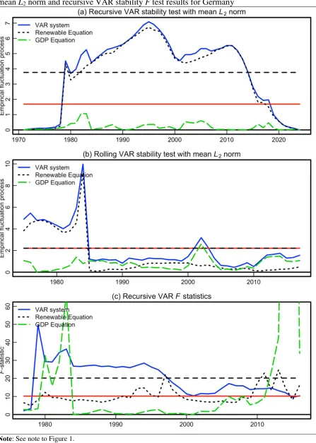
For the recursive and rolling-window parameter stability, we use three tests, namely recursive
VAR stability test with L2 norm of Hansen [22] and Nyblom [30], rolling VAR stability test
with mean L2 norm of Hansen [22] and Nyblom [30], and recursive VAR stability F test for
the renewable energy consumption equation, real GDP equation and the VAR model. The
estimation results for recursive and rolling-window parameter stability are reported in Figures
1-7. These analyses which use sup norm indicate that parameter stability for both individual
equations and VAR systems can be rejected. This means that we cannot reject a persistent
temporary deviation from the normal parameter levels. However, it can be rejected against a
single-break alternative. To sum up, in this analysis, the fact that the parameters of the VAR
models used for the G-7 countries are not stable. Thus, we use the HD method because of the
superior features of the historical decomposition method described above against other
methods used in the literature when the impact of the series on each other is time-varying.
Using the HD method, we could examine the cumulative effects of both renewable energy
consumption shocks on business cycle variation in real output and economic growth shocks
14 Figure 1: Recursive VAR stability test with mean L2 norm, rolling VAR stability test with mean L2 norm and recursive VAR stability F test results for Canada
Note: (a) Recursive VAR stability L2-test (b) Rolling VAR stability L2-test. (c) Recursive VAR stability F-test.
[image:15.595.71.522.100.658.2]15 Figure 2: Recursive VAR stability test with mean L2 norm, rolling VAR stability test with mean L2 norm and recursive VAR stability F test results for France
16 Figure 3: Recursive VAR stability test with mean L2 norm, rolling VAR stability test with mean L2 norm and recursive VAR stability F test results for Germany
[image:17.595.74.521.89.716.2]17 Figure 4: Recursive VAR stability test with mean L2 norm, rolling VAR stability test with mean L2 norm and recursive VAR stability F test results for Italy
[image:18.595.71.523.85.705.2]18 Figure 5: Recursive VAR stability test with mean L2 norm, rolling VAR stability test with mean L2 norm and recursive VAR stability F test results for Japan
[image:19.595.72.522.88.718.2]19 Figure 6: Recursive VAR stability test with mean L2 norm, rolling VAR stability test with mean L2 norm and recursive VAR stability F test results for UK
[image:20.595.73.523.90.707.2]20 Figure 7: Recursive VAR stability test with mean L2 norm, rolling VAR stability test with mean L2 norm and recursive VAR stability F test results for US
[image:21.595.70.522.87.705.2]21 Figure 8 provides the time series plot of the logarithm of renewable energy
consumption for the G-7 countries over the study period. The renewable energy consumption
follows a decreasingly growing trend in Canada. In Germany and Italy, renewable energy
consumption follows an increasing trend after flattening out until the early 1990s. In France
and United Kingdom, a completely different renewable energy consumption curve is
observed. For France, the slightly increasing consumption rate showed a drastic shift at the
end of the 1960s and has become stagnant since then. In the United Kingdom, a slight upward
trend was observed in renewable energy consumption from 1960 to the late 1980s, and then
this consumption showed a linear growing trend from the early 1990s with a big jump in
1987. Japan's graph of renewable energy consumption indicates that the consumption line
with a tendency to increase linearly throughout the whole analysis period appears to have
been broken at the beginning of the 1980s. Finally, the renewable energy consumption of
United States tracks the linear growing path up to 1985, and then it goes on a stagnant path
until it catches a linear growth tendency after 2000. The logarithm of the real GDP series is
plotted in Figure 9 for the G-7 countries. From 1960 to the present day, the real GDP growth
22 Figure 8: Time Series plot of the log of renewable energy consumption for the G-7 countries
0
(a) Canada
1960 1965 1970 1975 1980 1985 1990 1995 2000 2005 2010 2015 4.1
4.3 4.5 4.7
(c) Germany
1970 1973 1976 1979 1982 1985 1988 1991 1994 1997 2000 2003 2006 2009 2012 2015 3.4 3.6 3.8 4.0 4.2 4.4 4.6 (e) Japan
1960 1965 1970 1975 1980 1985 1990 1995 2000 2005 2010 2015 3.7
3.9 4.1 4.3
(g) United States
1960 1965 1970 1975 1980 1985 1990 1995 2000 2005 2010 2015 4.6 4.7 4.8 4.9 5.0 5.1 5.2 (b) France
1960 1965 1970 1975 1980 1985 1990 1995 2000 2005 2010 2015 3.4 3.6 3.8 4.0 4.2 4.4 (d) Italy
1960 1965 1970 1975 1980 1985 1990 1995 2000 2005 2010 2015 3.7
3.9 4.1 4.3 4.5
(f) United Kingdom
1960 1965 1970 1975 1980 1985 1990 1995 2000 2005 2010 2015 2.4
23 1
Figure 9: Time Series plot of the log of the real GDP series for the G-7 countries
(a) Canada
1960 1965 1970 1975 1980 1985 1990 1995 2000 2005 2010 2015 4.2 4.3 4.4 4.5 4.6 4.7 (c) Germany
1970 1973 1976 1979 1982 1985 1988 1991 1994 1997 2000 2003 2006 2009 2012 2015 4.25 4.35 4.45 4.55 4.65 (e) Japan
1960 1965 1970 1975 1980 1985 1990 1995 2000 2005 2010 2015 3.9
4.1 4.3 4.5 4.7
(g) United States
1960 1965 1970 1975 1980 1985 1990 1995 2000 2005 2010 2015 4.2 4.3 4.4 4.5 4.6 4.7 4.8 (b) France
1960 1965 1970 1975 1980 1985 1990 1995 2000 2005 2010 2015 4.1 4.2 4.3 4.4 4.5 4.6 4.7 (d) Italy
1960 1965 1970 1975 1980 1985 1990 1995 2000 2005 2010 2015 4.0 4.1 4.2 4.3 4.4 4.5 4.6
(f) United Kingdom
24 2
Figure 10 reports the estimates of economic growth shocks on renewable energy 3
consumption. 95% confidence intervals for the HDs are also given in each Figure. The 4
estimation results demonstrate that generally the effect of economic growth on renewable 5
energy is positive for all the G-7 countries during the analysis period. In Germany, Italy and 6
the United States, the effect of economic growth on renewable energy consumption is 7
significantly positive over the entire analysis period; while in other countries the contribution 8
of economic growth to renewable energy consumption is close to zero or gets even a negative 9
value in a few times. That is, energy conservation policies implemented in all the G-7 10
countries have become a very important tool in combating global warming. Moreover, the 11
effect of economic growth on renewable energy consumption is slightly increasing in Italy, 12
Japan and the United States, while this effect is decreasing in France and is stagnant in 13
Canada and Germany. Looking at the individual results for Japan, the contribution of 14
economic growth to renewable energy consumption fluctuates during the first and second oil 15
crises and then becomes stagnant after that period. To sum up, economic growth requires 16
renewable energy needs during all the analysis period for Germany, Italy and the United 17
States; on the other hand, it increases energy needs in other countries during all the analysis 18
period except for some short time intervals. 19
20
25 Figure 10: The effect of economic growth on renewable energy consumption
Note: The line in the middle represent the effect of the growth shock on the renwable energy consumption with surrandin lines representing the 95% confidence limits. Shaded refions denote the periods where the effect of the growth shock are postitive.
23
24
(a) Canada
1965 1970 1975 1980 1985 1990 1995 2000 2005 2010 2015 -0.02 -0.01 0.00 0.01 0.02 0.03 (c) Germany
1975 1978 1981 1984 1987 1990 1993 1996 1999 2002 2005 2008 2011 2014 0.00
0.02 0.04 0.06
(e ) Japan
1965 1970 1975 1980 1985 1990 1995 2000 2005 2010 2015 -0.03
-0.01 0.01 0.03
(g) Unite d States
1965 1970 1975 1980 1985 1990 1995 2000 2005 2010 2015 -0.010 0.000 0.010 0.020 0.030 (b) France
1965 1970 1975 1980 1985 1990 1995 2000 2005 2010 2015 -0.06 -0.02 0.02 0.06 0.10 (d) Italy
1965 1970 1975 1980 1985 1990 1995 2000 2005 2010 2015 -0.010
0.000 0.010 0.020 0.030
(f) Unite d Kingdom
1965 1970 1975 1980 1985 1990 1995 2000 2005 2010 2015 -0.04
26 Figure 11: The effect of renewable energy consumption on economic growth
Note: The line in the middle represent the effect of the renewable energy shock on economic growth with surrandin lines representing the 95% confidence limits. Shaded refions denote the periods where the effect of the renewable energy shocks are postitive.
(a) Canada
1965 1970 1975 1980 1985 1990 1995 2000 2005 2010 2015 -0.06
-0.02 0.02 0.06
(c) Germany
1975 1978 1981 1984 1987 1990 1993 1996 1999 2002 2005 2008 2011 2014 -0.075
-0.025 0.025 0.075
(e) Japan
1965 1970 1975 1980 1985 1990 1995 2000 2005 2010 2015 -0.10
-0.05 0.00 0.05 0.10 0.15
(g) United States
1965 1970 1975 1980 1985 1990 1995 2000 2005 2010 2015 -0.06
-0.02 0.02 0.06
(b) France
1965 1970 1975 1980 1985 1990 1995 2000 2005 2010 2015 -0.1
0.1 0.3 0.5
(d) Italy
1965 1970 1975 1980 1985 1990 1995 2000 2005 2010 2015 -0.050
0.000 0.050 0.100
(f) Unite d Kingdom
1965 1970 1975 1980 1985 1990 1995 2000 2005 2010 2015 -0.1
27 The estimation results for renewable energy consumption effect on economic growth
are shown in Figure 11. Findings about the effect of renewable energy consumption on
economic growth indicate that the relationship is not fixed in any G-7 country. In all G-7
countries, this relationship is time-varying over the study period. The weakening nexus from
renewable energy consumption to economic growth since the early 1980s started to rise again
in 1986 with a negative dip in Germany. During the 2008 Global Financial Crisis, the growth
theory lost its power again, but it has recovered after that time. Especially since the early
1990s, we can say that in Germany, the use of renewable energy is the driving force for
economic growth. A similar situation seems to be the case for Italy and the United Kingdom.
On the other hand, the estimation results show that in France, Japan and the United States,
this relationship follows a mixed path during the analysis period. In other words, we cannot
say that the growth theory works strongly in all periods, or at least for a certain period of time.
These results clearly show that the effect of renewable energy consumption on economic
growth varies over time. Unlike previous studies2, it is not possible to assume a constant
causality relationship throughout the analysis period for these countries.
4. Conclusion
This paper attempted to assess the time-varying effects of renewable energy consumption on
economic growth and vice versa for the G-7 countries. For this purpose, the analysis used the
historical decomposition approach to determine the relationship, and the bootstrap method to
compute confidence intervals. The previous literature used full sample econometric methods
to determine the causal nexus between renewable energy consumption and economic growth.
The major drawback of these studies is the assumption that the relationship between the
variables is constant over time. Our study fills the gap in the literature and allows us to make
policy implications by incorporating structural changes in the period of analysis with regards
to the relationship between renewable energy consumption and economic growth.
The estimation results provide clear evidence that the effect of economic growth on
renewable energy consumption is time-varying and positive in all the time periods for
Germany, Italy and the United States. For Canada, France, Japan and the United Kingdom,
the contribution of economic growth to renewable energy consumption is close to zero or
2 A few efforts estimated by full sample models such as Chang et al. [14] and Tugcu et al. [41] concludes the
28 even falls below horizontal line in some periods. In other words, the reported findings
substantially contradict the conservation hypothesis for all the G-7 countries in all the analysis
periods. Other findings regarding the effect of renewable energy consumption on economic
growth provide diverse results; that is, a positive shock in the consumption of renewable
energy on economic growth seems not to produce a prevailing outcome over the entire
analysis period. After the early 1990s, the use of renewable energy in Germany, Italy and
United Kingdom has become the driving force for economic growth except for a few time
intervals. It is conceivable for these countries to invest in renewable energy technologies or to
switch to renewable energy from fossil fuels in these time intervals. In other countries, there
is no evidence that the growth theory operates for a long period of time. For future research, it
would be interesting to investigate the time-varying effects of renewable energy consumption
29 References
[1] Adewuyi AO, Awodumi OB. Renewable and non-renewable energy-growth-emissions
linkages: Review of emerging trends with policy implications. Renewable and Sustainable Energy Reviews. 2017;69:275-91.
[2] Al-mulali U, Fereidouni HG, Lee JY, Sab CN. Examining the bi-directional long run
relationship between renewable energy consumption and GDP growth. Renewable and Sustainable Energy Reviews. 2013;22:209-22.
[3] Alper A, Oguz O. The role of renewable energy consumption in economic growth:
Evidence from asymmetric causality. Renewable and Sustainable Energy Reviews. 2016;60:953-9.
[4] Amri F. The relationship amongst energy consumption (renewable and
non-renewable), and GDP in Algeria. Renewable and Sustainable Energy Reviews. 2017 Sep 1;76:62-71.
[5] Andrews, D. W. K. Tests for parameter instability and structural change with
unknown change point, Econometrica. 1993;61: 821–56.
[6] Andrews, D.W. K. and Ploberger, W. Optimal tests when a nuisance parameter is
present only under the alternative, Econometrica. 1994;62: 1383–414.
[7] Apergis N, Payne JE. Renewable energy consumption and economic growth: evidence
from a panel of OECD countries. Energy policy. 2010;38(1):656-60.
[8] Apergis N, Payne JE. Renewable energy consumption and growth in Eurasia. Energy
Economics. 2010;32(6):1392-7.
[9] Azlina AA, Law SH, Mustapha NH. Dynamic linkages among transport energy
consumption, income and CO 2 emission in Malaysia. Energy Policy. 2014;73:598-606.
[10] Balcilar M, Ozdemir ZA, Arslanturk Y. Economic growth and energy consumption
causal nexus viewed through a bootstrap rolling window. Energy Economics. 2010;32(6):1398-410.
[11] Bhattacharya M, Paramati SR, Ozturk I, Bhattacharya S. The effect of renewable
energy consumption on economic growth: Evidence from top 38 countries. Applied Energy. 2016 Jan 15;162:733-41.
[12] Bildirici ME. The relationship between economic growth and biomass energy
consumption. Journal of Renewable and Sustainable Energy. 2012;4(2):023113.
[13] Burbidge J, Harrison A. An historical decomposition of the great depression to
determine the role of money. Journal of Monetary Economics. 1985 Jul 1;16(1):45-54.
[14] Chang T, Gupta R, Inglesi-Lotz R, Simo-Kengne B, Smithers D, Trembling A.
Renewable energy and growth: Evidence from heterogeneous panel of G7 countries using Granger causality. Renewable and Sustainable Energy Reviews. 2015;52:1405-12.
[15] Chien T, Hu JL. Renewable energy and macroeconomic efficiency of OECD and
non-OECD economies. Energy Policy. 2007;35(7):3606-15.
[16] Destek MA, Aslan A. Renewable and non-renewable energy consumption and
30
[17] Destek MA. Renewable energy consumption and economic growth in newly
industrialized countries: Evidence from asymmetric causality test. Renewable Energy. 2016 Sep 1;95:478-84.
[18] Efron B. The jackknife, the bootstrap and other resampling plans. Society for
industrial and applied mathematics; 1982.
[19] EUROSTAT, Renewable energy in the EU, 2017, available online at
(http://ec.europa.eu/eurostat/documents/2995521/7905983/8-14032017-BP-EN.pdf/af8b4671-fb2a-477b-b7cf-d9a28cb8beea.)
[20] Fang Y. Economic welfare impacts from renewable energy consumption: the China
experience. Renewable and Sustainable Energy Reviews. 2011;15(9):5120-8.
[21] Halkos GE, Tzeremes NG. The effect of electricity consumption from renewable
sources on countries׳ economic growth levels: Evidence from advanced, emerging and
developing economies. Renewable and Sustainable Energy Reviews. 2014 Nov 1;39:166-73.
[22] Hansen, B. E. Tests for parameter instability in regressions with I(1) processes.
Journal of Business and Economic Statistics. 1992;10: 321–36.
[23] Kahia M, Aïssa MS, Lanouar C. Renewable and non-renewable energy use-economic
growth nexus: The case of MENA Net Oil Importing Countries. Renewable and Sustainable Energy Reviews. 2017 May 1;71:127-40.
[24] Kahia M, Kadria M, Aissa MS, Lanouar C. Modelling the treatment effect of
renewable energy policies on economic growth: Evaluation from MENA countries. Journal of Cleaner Production. 2017;149:845-55.
[25] Kilian, L., Lütkepohl, H. The Relationship between VAR Models and Other
Macroeconometric Models. In Structural Vector Autoregressive Analysis (Themes in Modern Econometrics, pp. 171-195), 2017. Cambridge: Cambridge University Press. doi:10.1017/9781108164818.007
[26] Koçak E, Şarkgüneşi A. The renewable energy and economic growth nexus in Black
Sea and Balkan countries. Energy Policy. 2017;100:51-7.
[27] Lu WC. Renewable energy, carbon emissions, and economic growth in 24 Asian
countries: evidence from panel cointegration analysis. Environmental Science and Pollution Research. 2017 Nov 1;24(33):26006-15.
[28] Lütkepohl H. New introduction to multiple time series analysis. Springer Science &
Business Media; 2005.
[29] Menegaki AN. Growth and renewable energy in Europe: a random effect model with
evidence for neutrality hypothesis. Energy Economics. 2011;33(2):257-63.
[30] Nyblom, J. Testing for the constancy of parameters over time, Journal of the American
Statistical Association. 1989;84: 223–30.
[31] Ocal O, Aslan A. Renewable energy consumption–economic growth nexus in Turkey.
Renewable and Sustainable Energy Reviews. 2013;28:494-9.
[32] OECD. Renewable energy, available online at
(http://www.oecd-ilibrary.org/energy/renewable-energy/indicator/english_aac7c3f1-en).
[33] Phillips PC, Perron P. Testing for a unit root in time series regression. Biometrika.
31
[34] Phillips PC. Time series regression with a unit root. Econometrica: Journal of the
Econometric Society. 1987 Mar 1:277-301.
[35] Saad W, Taleb A. The causal relationship between renewable energy consumption and
economic growth: evidence from Europe. Clean Technologies and Environmental Policy. 2018 Jan 1:1-0.
[36] Sadorsky P. Renewable energy consumption and income in emerging economies.
Energy policy. 2009;37(10):4021-8.
[37] Saidi K, Mbarek MB. Nuclear energy, renewable energy, CO 2 emissions, and
economic growth for nine developed countries: Evidence from panel Granger causality tests. Progress in Nuclear Energy. 2016;88:364-74.
[38] Shahbaz M, Loganathan N, Zeshan M, Zaman K. Does renewable energy
consumption add in economic growth? An application of auto-regressive distributed lag model in Pakistan. Renewable and Sustainable Energy Reviews. 2015;44:576-85.
[39] Statistics, I.E.A. "CO2 emissions from fuel combustion-highlights, available online at
(https://www.iea.org/publications/freepublications/publication/CO2EmissionsFromFu elCombustionHighlights2015.pdf.)
[40] Troster V, Shahbaz M, Uddin GS. Renewable Energy, Oil Prices, and Economic
Activity: A Granger-causality in Quantiles Analysis. Energy Economics. 2018 Jan 31.
[41] Tugcu CT, Ozturk I, Aslan A. Renewable and non-renewable energy consumption and
economic growth relationship revisited: evidence from G7 countries. Energy economics. 2012;34(6):1942-50.
[42] World Bank. Gross Domestic Product (constant 2010 US$), available online at
(https://data.worldbank.org/indicator/NY.GDP.MKTP.KD).
[43] Yildirim E, Saraç Ş, Aslan A. Energy consumption and economic growth in the USA:
Evidence from renewable energy. Renewable and Sustainable Energy Reviews. 2012;16(9):6770-4.
[44] Zeileis A, Leisch F, Kleiber C, Hornik K. Monitoring Structural Change in Dynamic