2D PIV measurement on the interaction zone between two parallel planar jets in a crossflow

1_{Department of Mechanical and Manufacturing Engineering, Trinity College Dublin,}

University of Dublin, Ireland

2_{Energy and Power Technology Division, Department of Mechanical Engineering,}

University of Nigeria, Nsukka, Enugu 400001, Nigeria

(Received 26 May 2017; accepted 26 September 2017; published online 6 October 2017)

This paper reports an experimental investigation on the zone between two paral-lel planar jets in a crossflow, termed as the interaction zone. The experiment was conducted using 2D PIV measurement, which involves a test matrix designed for a parametric study. Based on both mean and instantaneous results, effects of dif-ferent parameters, i.e. front jet velocity, space between the two jets, and crossflow flow velocity, on the interaction zone were analysed. The two coupled recirculation structures, size, velocity field, and turbulence characteristics of the interaction zone are discussed. In addition, the large-scale vortices inside the interaction zone were recognised using Γ₁ value. How these different parameters affect the evolution of these vortices was also studied. ©2017 Author(s). All article content, except where otherwise noted, is licensed under a Creative Commons Attribution (CC BY) license (http://creativecommons.org/licenses/by/4.0/).https://doi.org/10.1063/1.5005017

I. INTRODUCTION

Tandem jets in a crossflow (TJCF) can be found in a number of engineering applications, e.g. lift jets of V/STOL aircraft, turbine blade cooling, and flow-induced noise reduction.1–3_{As a generic}

flow regime, extensive studies, especially in experiment4–15_{have been performed for both research}

and engineering interest. The performance of the jets has a great impact on the entire flow field. Therefore, the characterisation of the jets has become the main research area in TJCF.

Previous observations from the experiment5,7,11,13showed that when tandem jets, for example, dual jets are ejected into a crossflow, both of them will be deflected downstream. However, due to the shielding from the front jet, the crossflow momentum around the rear jet will be substantially reduced and therefore it will deflect less than the front jet. As a consequence, the two jets will gradually merge and finally combine into one. In addition to the defection, the shielding from the front jet has been found to have more impact on the rear jet, in terms of decay rate of the mean centerline velocity,12 jet spreading,12entrainment,14vortices,14etc.

When it comes to vortex dynamics, two groups of vortices16have been identified in the traverse jet in a crossflow. One group refer to those structures that are induced by the interaction among the jet, crossflow, and the wall, including Counter-Rotating Vortex Pair (CRVP), Horseshoe Vortices (HSV), Wall Vortices (WV) and Upright Vortices (UV). The other group consist of those structures that exist in the free jet as well, but whose evolution and destabilisation are influenced by the crossflow, e.g. Ring-Like Vortices (RLV).

One more characteristic that is worth mentioning is the recirculation zone below the rear jet. Discussions on the recirculation zone can be found in some studies on the single jet in the crossflow (SJCF).17–19In particular, due to the shielding from the jet, the ambient fluid in the trailing side of the jet loses its crossflow momentum and is entrained into the jet. The strong entrainment quickly transports fluid that is close to the trailing edge of the jet, inducing pressure gradient. This gradient has

a

[email protected]

understanding of the entire flow field, more discussion on other areas is worth conducting.

The present study investigates an interesting region between two planar jets in the crossflow ambient. Since the development of this region is highly dependent on the interaction of the two jets, this region is termed as the interaction zone (IZ). Based on the 2D-PIV measurement, a parametric analysis was conducted to compare the effects on the IZ. Both mean and instantaneous results are reported in this paper, encompassing two coupled recirculation structures, velocity field, turbulence characteristics and large-scale vortices.

II. EXPERIMENTAL APPARATUS

Experiments were carried out in a subsonic open-jet wind tunnel. All measurements were made using a low-speed 2D-PIV system.

A. Wind tunnel system

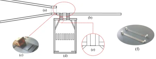
The wind tunnel system used in this study consists of a subsonic open-jet wind tunnel, a test platform, and a planar jet generator, described in Fig.1. The entire system was supported by aluminium extrusion frame.

The subsonic open-jet wind tunnel was used to create a crossflow up to 70 m/s, powered by a 5.5kW centrifugal blower. The nozzle of the tunnel, as illustrated in Fig.1(a), was connected to a cubic plenum upstream, with a size of 800mm×800mm×800mm. The plenum can uncouple flow from the blower, pressurise the air, and suppress the turbulence level through two layers of mesh plate inside. The nozzle, with an outlet size of 75mm×75mm, was made to be flush with a horizontal end-plate, shown in Fig.1(b). On the endplate, two planar jet slots were installed, the configuration of which can be found in Fig.1(c).

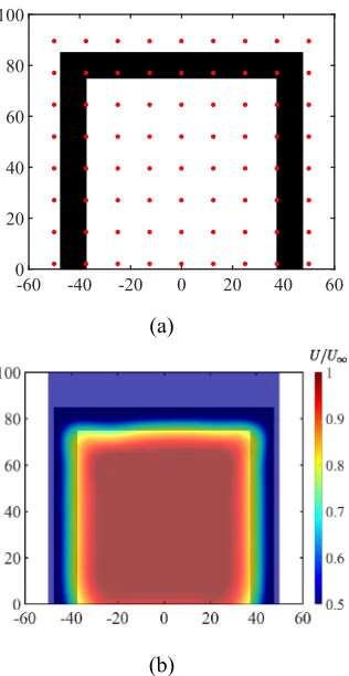
The crossflow ejected from the nozzle of the wind tunnel has been characterised using the hot-wire anemometry. The probe was a single-hot-wire Dantec 55P15.23_{As schematically shown in Fig.2(a),}

a few sampling points were planned outside the nozzle of the crossflow, on which the measurement of the velocity was conducted. More specifically, the black shade illustrates the nozzle exit in scale. The bottom row of the sampling points are 2mm higher than the end-plate, and the distance between each row is 12.5mm. Based on the interpolation of the measurement results, the velocity profile of the crossflow nozzle can be achieved. In Fig.2(b), the profile is reported as the contour superimposed on the nozzle exit, normalised by the maximum velocity in the profile. In this case,U∞=30.199 m/s.

Note that the crossflow and the jet velocities reported in this paper, i.e.U∞,U1, and U2, are the

FIG. 2. Characterisation of the velocity profile of the crossflow nozzle using the hot-wire anemometry. (a) Sampling point; (b) Velocity prole of the crossow nozzle.

maximum velocity in the profile. Since the measurement was conducted in the centre-plane of the crossflow, the velocity profile is also reported in Fig.3. It is observed that there are three shear layers on the top, right and left sides of the crossflow, respectively. The shear layers on the right and left sides on the jet in the PIV measurement window can be ignored since the measurement was conducted in the centre-plane. This will be further described in SectionII B. As for the upper shear layer, the entire crossflow as well as the upper shear layer will be defected by the jet. Therefore, it will not interact with the planar jet. The turbulence intensity of the streamwise component below the upper shear layer of the crossflow is within 1%.

The planar jet generator comprises a 2.2kW centrifugal blower, a cubic plenum and the two jet slots. A hose was linked from the blower outlet to the bottom of the plenum. As described in Fig.1(d), the plenum was situated below the endplate and had a height of 540mm. The horizontal cross-section of the plenum is 424mm×424mm. Likewise, to reduce the turbulence level of the jets, one layer of honeycomb with a hexagonal grid (6mmedge length) was mounted in the middle of the plenum.

FIG. 4. Normalised jet exit velocity profiles in the centre-plane.

Additionally, baffles were added to suppress recirculation. The two parallel jet slots were connected on the top of the plenum, the width (4) of which was 10mm and the spanwise length of the jet was 100mm. Note thatP, i.e. centre-to-centre space between the two jets, can be altered as required. The value will be reported later in SectionII C. Considering the plenum was shared by the two jets, a special mechanism was adopted to manipulate the jet speeds independently. More specifically, in the junction between the font jet and the plenum, one thin mesh plate was installed, as schematically described in Fig.1(e). The alloy mesh plate was designed with a variety of porosity. By changing the mesh plate and adjusting the actual power of the blower, the required speeds can be acquired for the two jets. Examples of the alloy mesh plate are given in Fig.1(f). In the test program, only three jet velocities were used, i.e. 37m/s, 25m/s and 13m/s. The velocity profiles in the centre-plane of the jet has also been characterised by the hot-wire, reported in Fig.4.

B. PIV arrangement

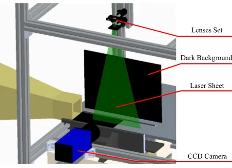
A 2-D low-speed PIV system was used to carry out all flow measurements, which allow a quantitative analysis of the flow regime. To visualise the flow field, both the jets and the crossflow were seeded with Pea Soup®Oil Based Smoke Generator PS31. The size of the particle was in the order of 1.5µm. The measurement plane was made to align with the centre-plane of the test section, which is also the farthest section to the corner. This contributes to the 2D representation of the flow field. Particles in the plane were illuminated using a sharp laser sheet. The source of the sheet was a New Wave Solo-II PIV double pulsed Nd:YAG laser (532 nm, 30 mJ/pulse), mounted on the top of the aluminium frame. One lens set was used to diverge the point source to a line source. In addition, in order to highlight the illuminated plane, one black PVC board was fixed behind the laser sheet as a dark background. Note that the board was outside the crossflow and accordingly had no interference

FIG. 6. Schematic of dual planar jets set-up.

with the flow. A LaVision®FlowMaster CCD camera was situated beside the test section, taking image pairs of the flow field of interest. A 532 nm narrowband pass optical filter was installed to the camera lens in the measurement. 3D CAD sketch of the PIV arrangement is shown in Fig.5. The image pairs were captured at 4 frames per second, and the time delay between two images in one pair was 15µs. The resolution of the CCD camera is 1280 pixels by 1024 pixels. In the set-up described above, the image size was 106 mm×84.6 mm (X×Y). This allows the image to have a resolution of 12 pixels×12 pixels per mm2_{. Those image pairs were processed using cross-correlation in DaVis®}

software with decreasing multi-pass interrogation window sizes, 32×32 and 16×16, respectively. There were two passes and 50% overlap in each window size. The post-processing was performed with an open access Matlab toolbox-PIVMat.24

C. Test programme

The test programme in this study was designed to study the effects of different parameters on the IZ. Fig.6is a schematic of the dual-jet configuration, along with a 2-D Cartesian coordinate system utilised throughout this paper. In this system, the origin of the system aligns with the centre of the rear jet outlet, with theXaxis along the streamwise direction andY normal to end-plate. Note that in all test cases, the rear jet position, with the reference to the crossflow nozzle, was fixed, i.e.l= 195mm. By contrast, the front jet was installed with different distancesPfrom the rear jet.

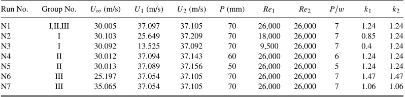
Parameters of each case in the test programme are tabulated in TableI. The velocity of the jet and crossflow was measured using an FCO510 Micromanometer equipped with a Pitot tube. Herein, the blowing ratio (k1andk2) is introduced. In the study of SJIC, the blowing ratio is usually defined

TABLE I. PIV test matrix.

Run No. Group No. U∞(m/s) U1(m/s) U2(m/s) P(mm) Re1 Re2 P4 k1 k2

N1 I,II,III 30.005 37.097 37.105 70 26,000 26,000 7 1.24 1.24

N2 I 30.103 25.649 37.209 70 18,000 26,000 7 0.85 1.24

N3 I 30.092 13.525 37.092 70 9,500 26,000 7 0.4 1.24

N4 II 30.012 37.094 37.143 60 26,000 26,000 6 1.24 1.24

N5 II 30.013 37.089 37.156 50 26,000 26,000 5 1.24 1.24

FIG. 7. Validation of the 2D characteristic.

as the ratio of the jet velocity to the local crossflow velocity. However, due to the shielding from the front jet, the local crossflow velocity of the rear jet is no longerU∞. In this paper,k2is still defined

asU2U∞, which is the nominal blowing ratio of the rear jet. It is certain that the real blowing ratio

of the rear jet is much greater thank2.

As shown in Table I, each test case has been identified by a Run Number. These cases can be divided into three parametric groups, in which N1 is the baseline case. In Group I, N1, N2 and N3 have differentU1(andRe1 andk1), they are compared to study the effects on the IZ from the

front jet velocity. In Group II, N1, N4 and N5 were installed with differentP (andP

4), used to analyse the effects from the space between the jets. Group III have N1, N6 and N7. In this group, the two jets were ejected into different crossflow velocities, which can investigate the effects from differentU∞.

In order to reach convergence of the mean properties, 1,500 image pairs were acquired for each case in the test matrix. In the mean flow field of all cases, the maximum uncertainty was found to be ±0.017 m/s.

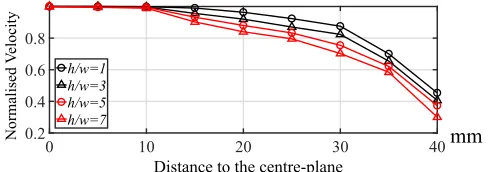
Due to the shear layer on the sides of the crossflow, and the low aspect-ratio of the planar jet outlet, it is necessary to validate the 2D performance of the flow in the measurement range. Here we introduce a simple approach based on hot-wire measurement. This approach used similar sampling method in the crossflow velocity characterisation, shown in Fig.2(a). However, due to the symmetry regarding the centre-plane, the data sampling was only conducted on the one side of the centre-plan. What is more, the sampling section is close to the downstream limit of the PIV window, instead of the the crossflow nozzle. This is because the flow spread more in the downstream than the upstream. Therefore, if the 2D performance is guaranteed downstream, the upstream flow will be also 2D. Here

his used to term the height of the sampling point row, the sampling was taken ath

4= 1,h 4= 3,

h

4= 5, andh

4= 7, respectively. In each row, there are 9 sampling point with different distance to the centre-plane. The velocity profiles are reported in Fig.7, normalised by the centre-plane velocity. It is found that the velocity almost keeps the magnitude within a distance of 10mm. As such, it is sensible to say that the flow within the measurement plane, i.e. the centre-plane is two dimensional and we can proceed to the following discussion.

III. RESULTS AND DISCUSSION

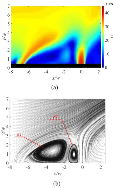
FIG. 8. Mean flow field of N1. (a) Velocity contour; (b) Streamline.

asR2. In this section, study onR1 andR2 is reported. Also, the large-scale vortices inside the IZ are discussed.

A. Coupled recirculation structures

R1 andR2 are two full recirculation structures that can be detected in the mean streamline field of the IZ. It is worth mentioning that research work by Gutmark et al.12_{also observed the streamlines of}

two circular jets in a crossflow. However, despite the existence of recirculation, no such full structure was found due to the 3D configuration. As such,R1 andR2 can be recognised as a unique characteristic of the planar TJIC.

1. Formation of R1 and R2

The formation ofR1 andR2 is highly correlated to the jet entrainment of the ambient fluid. Fig.9 shows the vector field of the IZ, it is clearly shown that the rotation direction ofR1 andR2 is clockwise and counter-clockwise, respectively. ForR1, when the front jet is discharged, the crossflow momentum inside the IZ will be shielded. As a consequence, the relatively quiescent fluid in the trailing proximity of the front jet will be continuously entrained into the jet, inducing a pressure gradient. Due to the 2-D characters of the planar jet, this gradient has to be offset by the fluid downstream, which in turn will also lead to new pressure gradient herein and drag down the fluid from the upper side of the IZ. Therefore,R1 is established with a clockwise rotation. As mentioned in SectionI, in SJIC a large recirculation zone can be also observed downstream to the jet.17–19As such,R1 corresponds to the same recirculation structure of the front jet, but confined inside the IZ by the rear jet.

FIG. 9. Velocity vector field and sketch of the recirculation structures.

In the 2D field, the roll-up of the HSV will be substantially enhanced. Due to the time-dependent periodicity,27a recirculation zone in the mean flow field will establish in the leading side of the jet slot, with a contour-clockwise rotation. In the IZ of TJIC, the upstream recirculation zone of the rear jet extends due to the reduced crossflow momentum. As such, it develops toR2 in the mean flow field. This also explains why the recirculation structures can be also observed upstream to the front jet. For example, in Fig.10(e), the recirculation structure can be also observed upstream to the front jet, but with a much smaller size. This is because the downward portion ofR1 and the upward velocity of the rear jet contributes to a continuous pressure gradient aroundR2. This gradient enhancesR2 and makes it much larger.

One more important aspect ofR1 andR2 that is related to their formation is the coupling. To be more specific, the pressure gradient that drags down the fluid from the upper side of the IZ, couplesR1 andR2. On one hand, the downward flow plays a role as the boundary to confine the relative position of the two structures. As a result,R1 andR2 have to be situated on each side of the IZ respectively. On the other hand, the downward flow is the edge shared byR1 andR2. Therefore,R1 andR2 are highly coupled with mutual effects.

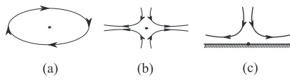
FIG. 11. Critical points in the flow field. (a) Centre; (b) Saddle; (c) Reattachement.

2. Critical points and area of R1 and R2

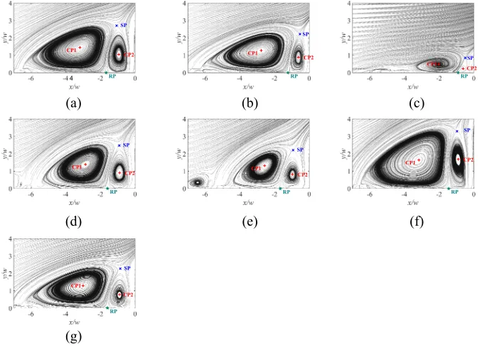
Fig.10reports the mean streamline field in the IZ from all test cases. Overall, it appears that

R1 is dominant overR2 in terms of the size. Besides, the area and the position ofR1 andR2 vary with the parameters of the flow field. As such, in order to characterise the two coupled recirculation structures,R1 andR2 are quantitatively investigated from a topological point of view: the critical points and the size of the structures are compared, as a parametric analysis.

In the mean flow field, a critical point is a position where the velocity vanishes. For example, Fig.11 shows three typical critical points inside 2D flow streamlines: centre point, saddle point, and reattachment point. To be more specific, the centre point is the pivot around which streamlines revolve; the stagnation point is where streamlines from different directions converge and then leave in other directions; the reattachment point is the stagnation point on the wall. In the streamline field, the location of the critical point can be determined using Taylor serious and the standard theory for Hamiltonian systems.28–30

The coordinates of the critical points are calculated and illustrated in Fig.10. One centre point is found within each recirculation structures, and CP1 and CP2 are used to denote them respectively. One stagnation point, termed as SP, can be detected in the region where the front jet, the rear jet,R1, andR2 converge. On the end-plate, there exists one reattachment point betweenR1 andR2, denoted as RP. Because CP1 and CP2 are the centre point of the two recirculation structures, they can be used to assess the locus ofR1 andR2’s motion. The stagnation point is where the streamlines of the jets and the recirculation structures converge, SP can be treated as the combining point of the two jets, viz. the upper limit of the IZ. As for RP, it is used to separateR1 andR2 and accordingly applied for the area calculation, introduced later in this same section.

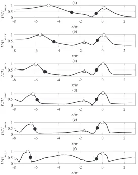
In order to characterise the recirculation structures, the area is an important characteristic, which needs to be first addressed. Obviously, RP is the lower limit. Regarding the edge, they are recognised in this paper based on the velocity magnitude profile along the horizontal direction. More specifically,

FIG. 13. Velocity magnitude profiles of N1 acquired along the horizontal direction at (a)y

4= 2.4; (b)y

4= 1.8; (c)y

4= 1.4; (d)y

4= 1; (e)y

4= 0.8; (f)y

4= 0.2. Note thatUmaxis the maximum velocity magnitude in each profile.

Fig.12is the schematic of the two jets, with a magnification view of the IZ. A number of horizontal lines between SP and the end-plate are made to extract velocity magnitude profiles from the IZ. In Fig. 13, examples of the velocity profiles from N1 at different y₄

are shown. It is observed that two peaks coexist in each profile (highlighted with the empty circle◦), which can be reasonably attributed to the centreline of the jet, and the IZ is between them. Considering the width and spreading of the jet, the locus of the half magnitude point of each peak in the sampling profile is used to be the boundary between the jet and the IZ (highlighted with the solid circle •). Obviously, when

y₄

= 0, i.e. on the end-plate, the boundary begins at the trailing edge of the front slot and the

close to the SP. For example, those points marked with∆in the profiles of Fig.13(b)–(e). In fact, they are the location of the maximum downward velocity between R1 andR2. They are used for defining the shared edge ofR1 andR2, along with SP and RP. Fig.14shows the boundaries defined using the approach described above, superimposed on the streamlines. It is shown that the edges between the IZ agree well with the outside streamlines of the recirculation zone. The shared edge betweenR1 andR2 also separatesR1 andR2. Therefore, this definition can be used in the following analysis.

FIG. 16. Area ofR1,R2 and the IZ (42_{is the unit area, i.e.4×4).}

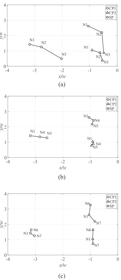
As a parametric study, it is observed from Fig. 10that the position of CP1, CP2 and SP is dependent on the flow conditions, so is the area of R1 andR2. To analyse the dependence, the coordinates of these three critical points are reported in the diagram in Fig.15; the area ofR1,R2, and IZ (discussed in SectionIII B), calculated using numerical integration, is reported in the bar chart in Fig.16.

Fig.15(a)illustrates the variation of the key points with the front jet velocityU1. It is found that

whenU1 becomes smaller, all three key points descend and in the meanwhile, move downstream.

Regarding the area, Fig.16(a)shows that both areas ofR1 andR2 become smaller. This trend can be further confirmed from the streamlines in Fig.10(a)–(c). Therefore, it is concluded that with the decrease ofU1, bothR1 andR2 will shrink and approach the rear jet slot proximity. In addition, the

two jets will combine at a lower and more downstream location. All of the variations can be simply explained by the reduced shielding from the front jet. When the front jet has less momentum, the shielding it provides to the rear jet will be less, therefore the rear jet will deflect more. Thus, SP becomes not just lower but also more downstream. Also,R1 andR2 have to cut down their size and move downstream due to a compressed IZ. For example, both R1 and R2 become extremely small in N3 in Fig.10(c), which has the lowestU1.

Fig.15(b)and Fig.16(b)describe the effects from the jet spaceP. It is observed that whenP

shortens, all of CP1, CP2 and SP gradually decrease. This is due to the reduction in the size ofR1 andR2. As shown in Fig.10(a),(d)and(e), whenP₄

to the rear jet in terms of both SP and CP2. One more interesting thing is the upstream recirculation zone of the front jet, observed from the front jet in Fig.10(d)and(e). Particularly, whenP

4= 5 in Fig.10(e), there is a full structure upstream of the front jet. It is worth noting that in other cases, there must be a similar structure existing upstream to the front jet. However, due to the limit of the PIV image range, it is not shown in other figures. As mentioned in SectionIII A 1, this one is a variation of the horseshoe vortices in the mean flow field, which corresponds toR2 within the IZ. Therefore, it is assumed that this recirculation structure exists in all front jets outside the image.

Fig.15(c)and Fig.16(c)illustrate the change of the key points and the recirculation areas with the crossflow velocityU∞. Obviously, a lowerU∞influences the size ofR1 andR2, and the height of

the centres. Also, the combination location of the two jets, SP will ascend to a higher position with a lowerU∞. However, similar to the effects fromP, the horizontal position of these key points do not

move with a uniform trend as the crossflow velocity reduces.

B. Size of the interaction zone

The size of the interaction zone is an important characteristic that is worth considering. As depicted in Fig.10, it is correlated with the investigating parameter. Here, the area of IZ was calculated as the sum ofR1 andR2.

As Fig.16shows, the total area of the IZ is dependent on toU1,PandU∞, which agrees with

Fig.10. Within the range being tested, it is obvious that the area of the IZ is positively corrected withU₁andP, but negatively withU∞. Furthermore, there are some extreme conditions that can be

discussed without the test. For example,U1→0\∞,P→0\∞,U∞→0\∞, respectively.

WhenU1→0, the scenario is similar to SJIC. Therefore,R1→0, butR2 will restore to be the

upstream recirculation of SJIC. Then the area of the IZ is equal to the upstream recirculation, termed asΩhere in after. Note that for a particularP, whenU1increases but is still small, the front jet may

directly merge with the crossflow ambient. This means that the front jet has little impact on the rear jet and the size of the IZ remains to be as same asΩ. But the size will be greater thanΩwhen the front jet velocity is sufficiently high and it starts to interact wit the rear jet. WhenU1→ ∞, this extreme

condition will extend the potential core of the front jet to an infinity long distance, and the shear layer in both trailing and leading sides become so thin that can be ignored. Therefore, little spreading will happen to the front jet. More importantly, such powerful front jet will completely block the crossflow. Moreover, the entrainment of the fluid from the IZ plays a crucial role, inducing pressure gradient to drag the rear jet close to the front jet. It is reasonable to infer that this drag is overwhelmingly strong and can directly deflect the rear jet, which means the size of the IZ will go to zero. As such, it is expected that whenU1increases from 0 to∞, there exists a peak value for the size of the IZ. The size

will firstly remain to be equal toΩ, and then start to increase until it reaches the peak. Subsequently, it declines and gradually approaches zero.

WhenP→0, obviously the IZ will disappear with no area. AsPincreases, the size of the IZ will at first increase, shown Fig.16(b). However, it is expected that whenP→ ∞, the front jet will have merged with the crossflow before making an influence on the rear jet, making the rear jet behave like the SJIC. The limit isΩas well. Therefore, it is concluded that a peak also exists whenPmoves from 0 to∞. Firstly, the area of the IZ remains to beΩuntil the front jet begins to interact with the rear jet. Then it will ascend to the peak and likewise, start to descend till zero.

WhenU∞→0, the dual jets will be ejected into a quiescent ambient. Previous studies31–33on the

dual moderately-spaced jets in a quiescent ambient reported that after ejection, two jets will merge and combine into one due to the mutual entrainment of each other. More importantly, a recirculation zone will show up between them. This can be the upper limit of the IZ size whenU∞→0. Furthermore,

it is easy to obtain the lower limit of the IZ regarding the crossflow velocity, i.e. the area of the IZ whenU∞→ ∞. Obviously, when such extreme condition happens, both jets will deflect immediately

after ejection, which means the area goes to zero. As such, unlikeU1andP, it is expected that area

FIG. 17. Mean velocity contour of the IZ. (a) N1; (b) N2; (c) N3; (d) N4; (e) N5; (f) N6; (g) N7.

C. Velocity field and turbulence proprieties

As shown earlier in Fig.8(a), there exists interesting characteristics in the velocity contour of the IZ, which are discussed in detail in this section. For ease of comparison, the contour with lines of the velocity field is illustrated in Fig.17, along with CP1, CP2 and SP. BecauseU2is constant in

all cases, the contour has been normalised by the rear jet velocity. It is observed that the magnitude around the three key points is the lowest within the IZ (U_U

2<0.1 ), which agrees with the definition

in SectionIII A 2. The low-speed region around CP1, denoted as LSRCP1, extends from the front

jet trailing proximity to the middle of the IZ. It is obvious that this region is the core area of R1. Likewise, the low-speed region around CP2, denoted as LSRCP2is the core area ofR2, close to the

front jet. Another low-speed region, which has the maximum height, is situated around the stagnation point SP, denoted as LSRSP. This is because the velocities from different directions cancel out here,

making SP surrounded with slow velocity magnitude. Note that in LSRCP1and LSRSP, the velocity

magnitude is less that 0.1U2. This allows the boundary to align with the contour line so that the

analysis can proceed.

In the middle of LSRCP1, LSRCP2and LSRSP, there exists an elliptic high-speed region, where

0.2<U_U

2<0.3. If compared with the streamlines in Fig.10, the high-speed region is attributed

to the shared edge of R1 andR2. More specifically, the two recirculation structures co-flow here, which accordingly raises the velocity magnitude. This high-speed region also separates LSRCP1

from LSRCP2 and LSRSP. The area of this high-speed region is also dependent on the flow initial

conditions. As for the separation between LSRCP2and LSRSP, it is found to be the upper portion of

R2. However, this separation is ambiguous. As shown in Fig.17(a)–(c), whenU1reduces, LSRCP2

and LSRSPtend to merge into one. From Fig.17(a),(f)and(g), it is found that whenU∞becomes

the lowest among the three cases, LSRCP2and LSRSPalso merge. However, the comparison among

Fig.17(a),(d)and(e)shows thatPhas less effect on the separation between LSRCP2 and LSRSP.

Therefore, it suggests that the recirculation speed ofR2 is dependent onU1andU∞, but less dependent

onP.

The mean characteristics of the turbulence are also analysed through the turbulence kinetic energy (TKE). In Fig. 18, the contour of TKE, normalised by the power of the rear jet velocity (TKE_U2

2) is illustrated, along with SP, CP1 and CP2. Also, TKE aty

₄

= 1 andy₄

FIG. 18. Turbulence kinetic energy of the IZ. (a) N1; (b) N2; (c) N3; (d) N4; (e) N5; (f) N6; (g) N7.

these two shear layers is evident. It can be observed in Fig. 18, especially (d) and (e), that the leading shear layer is more turbulent than the trailing one when close to the end-plate. However, the trailing one, which is more related to the interaction zone, can develop farther and blend into the peak region. This is because the leading shear layer is directly exposed to the crossflow. As a result, when the crossflow momentum is stronger than the jet, the vortices with different scale sizes in the upstream shear layer, which contributes to the growth of the TKE, will be suppressed. At last, the shear layer merges with the deflected crossflow with low TKE. By contrast, the trailing shear layer close to the IZ is shielded, which benefits a farther spread. This conclusion can be confirmed by Fig. 18(b) and(c), when the front jet velocity is low, hardly can the high TKE region in the leading shear layer be observed. On the development of the vortices in the upstream shear layer of the front jet, more detail will be discussed in SectionIII D. It is worth noting that in Fig.18(d)and(e), some high TKE can be found even ahead of the leading shear layer of the front jet. As mentioned earlier in SectionIII A 1, here is where the HSV develop. In terms of the mean field, there exists an upstream recirculation zone due to the front jet. As such, fluid here is more turbulent so that TKE increases.

All contour in Fig. 18shows that the peak zone of TKE is on the right side of SP, where, if referred to the streamlines in Fig. 10, the front jet strongly impinges the rear jet. This is under-standable because this area is characterised by instability. The area with the lowest TKE (dark blue colour in the contour) inside the IZ appears to be in the proximity of the front jet outlet. Like-wise, this is due to the shielding from the front jet. The fluid here approximates to be quiescent and therefore, is much less turbulent. This suggests that the more the shielding is, the larger the low TKE area will be. Since the shielding given by the front jet increases with a greaterU1, and

a lessU∞, it means that the low TKE area turns larger when the front jet velocity become higher,

confirmed by Fig. 18(a)–(c). Also, when the crossflow velocity decreases, the low TKE area is expected to be larger, shown in Fig.18(a),(f)and(g). As forP, whenPis reduced, because the entire IZ reduces, from Fig.18(a),(d)and(e), it is found that the low TKE area shows the same trend.

D. Large-scale vortices

FIG. 19. TKE profiles aty_{4= 1 andy4= 2. (a) Group I(N1, N2 and N3); (b) Group II(N1, N4 and N5); (c) Group III(N6,}

N1 and N7).

the development of the jet, e.g. dispersion and mixing of the fluids, noise production, combustion.34–36 As previously mentioned in SectionI, those large-scale vortices include, in reference to a circular jet, CRVP, HSV, WV, UV, and RLV.16Due to the approximately 2-D character, the main flow feature of a planar jet is the RLV. However, since the shape does not resemble a ring, it is termed as a Shear Layer Vortices (SLV) in the planar jet.21_{In this section, the large-scale vortices within the interaction}

zone is discussed, i.e SLV.

1. Recognition of the large-scale vortices

M∈S M

=1

S

S

sinθMdS,

(1)

whereAMis the radius vector, pointing fromAtoM,UMis the local velocity atM,θmis the angle

betweenAMandUM, andzis the normal unit vector to the plane. If applied for PIV measurements,

theΓ1value in the discrete vector field can be calculated as:

Γ1(A)=

1

N

X

S

AM×UM·z

|AM| · |UM|

=1

S

X

S

sinθM,

(2)

whereN is the number of pointM withinS. According to Graftieaux et al,37N plays the role of a spatial filter, which can be adjusted to locate large-scale vortices. However, N almost does not affect Γ₁ value of a vortex centre. After a few attempts N was used as 15 in this study. For all pointsΓ₁drops within the range between -1 and 1. Typically,|Γ₁|>2π

(≈0.637) corresponds to a presence of large-scale vortex,38and whetherΓ₁is positive or negative corresponds to the clockwise or counter-clockwise rotation.

In Fig.20, examples of the instantaneous velocity field from N1 at different time are shown, along with the |Γ1| contour superimposed. As a large-scale vortex detector,|Γ1|>2πwell locates those

vor-tices in each field. It is observed from all 1,500 results that the large-scale vorvor-tices only develop along the trailing edge of the front jet within the IZ, leading edge of the rear jet within the IZ, and trailing edge of the rear jet. However, no such structures exist on the leading edge of the front jet. As mentioned in SectionIII C, this can be attributed to the crossflow momentum. More specifically, when two jets are discharged, the front jet is directly exposed to the crossflow with a much larger momentum. Therefore, even though those eddies initially occur due to the shear layer instability in the leading edge of the front jet, the high-velocity gradient will quickly tear them up and transform them into small eddies. By contrast, with the shielding from the front jet, the crossflow momentum can be significantly reduced inside the IZ. This allows the large eddies to evolve before the two jets combine. Likewise, these large-scale eddies can be also found in the trailing edge of the rear jet, due to the shielding from both jets. In terms of the rotation direction, also found from the local vector field around the areas of|Γ₁|>2π

that those vortices in all trailing edges mentioned above are clockwise, and those in the leading edges, are counter-clockwise.

2. Evolution of the large-scale vortices

The Γ1 value also makes it possible to evaluate the size of the large-scale vortices, which is

defined as the total area around a core, where|Γ1|>2πin an instantaneous flow field. In this paper,

the counter-clockwise vortices from the leading edge of the rear jet are calculated as an exam-ple. However, the evolution of an eddy includes formation, growth and finally fracture into more eddies with smaller sizes, which means the size of an eddy rapidly varies. Due to the limitation of the PIV sampling frequency, it is impossible to capture the entire process of an eddy‘s evolution. Therefore, in order to obtain a parametric analysis on the size of counter-clockwise vortices, the probability of the size in statistics from all instantaneous results is adopted. As mentioned earlier, A positive or negative value ofΓ₁corresponds to a different rotation direction of an eddy, respec-tively. Here the negative one is considered to reckon the counter-clockwise vortices in the leading edge of the rear jet. First of all, those areas with |Γ₁|>2π

were recognised in from all 1,500 results. Among these 1,500 images, within 1%of them did not capture any counter-clockwise eddies. These results were eliminated from the total samples. Secondly, the size of the eddies based on −1<Γ₁<−2π

FIG. 20. Examples of instantaneous vector fields from N1, withΓ1contour superimposed.

1842-2042. Here those large-scale eddies are subdivided into thee categories with different sizes: 0-242and 242-642are treated as the small-size eddies; 642-1042and 1042-1442are the medium-size eddies, 1442-1842, and 1842-2042are the great-size eddies. The probability of each group is shown as a histogram in Fig. 21. Compared with other probabilities, those great-size eddies, especially 1842-2042, are much lower and cannot be clearly visualised. Therefore a zoomed sub-figure is made in each figure.

In Fig.21, N1 is used as the baseline and is shown in all cases with a consistent legend. Fig.21(a) describes probability variation against the rear jet velocity. It is found that when the front jet velocity reduces, the size of the large-scale vortices tends to shrink. In N3, which has the lowestU1, among

FIG. 21. Probability density histograms of the large-scale vortices size. (a) Group I(N1, N2, N3); (b) Group II(N1, N4, N5); (c) Group III(N6, N1, N7).

eddies also increases. Therefore, it is concluded that a higher front jet velocity can contribute to the evolution of the large-scale eddies in the leading edge of the rear jet.

Fig.21(b)illustrates the probability variation as a function of the space between two jets (P). Regardless of the value ofP, the large-scale vortices can be observed with all different sizes. In other world, within the test range, no obvious correlation between the vortex evolution andPcan be found. In Fig. 21(c), N1, N6, and N7 are compared to analyse the vortex size as a function of the crossflow velocity. Similarly, toU1, the crossflow velocity is correlated with the vortex size. When

the crossflow velocity increases from N7 to N1, then eventually N6, the probability of the great-size eddies reduces. For example, no great-size eddies can be detected in N7, which has the highestU∞.

such, the evolution of the large-scale vortices can have more space to proceed, thus, more great-size eddies will occur.

IV. CONCLUSIONS

In this paper, a 2D PIV measurement of the interaction zone between two planar jets was conducted. Both mean and instantaneous flow field results were reported. Based on the data, dis-cussions were made on the characterisation of the IZ, i.e. the two coupled recirculation structures, size, velocity and turbulence field of the IZ. Finally, an analysis of the large-scale vortices was conducted.

For the coupled recirculation structures, the formation ofR1 andR2 was firstly discussed. Com-pared with SJIC, it is concluded thatR1 corresponds to the downstream recirculation zone of the single jet, andR2corresponds to the upstream recirculation zone of the single jet. Secondly, an analysis of R1 andR2 was made, from a topological perspective, on the critical points and the area. The critical points include two centre points (CP1 and CP2), one stagnation point (SP), and one reattachment point (RP). CP1 and CP2 were taken to assess the position of the recirculation structures, SP was used to be the converging point of the two jets and the height of the IZ, and RP was used to be the lower limit of the boundary betweenR1 andR2. It is found that the position of the two recirculation structures and the converging point of the two jets varies with different parameters, which, the area ofR1 andR2 are also dependent on.

The size of the IZ was defined as the sum ofR1 andR2, calculated for all cases in the test matrix. Within the range tested, the size was observed to increase with the front jet velocity and the space between two jets. However, it is negatively correlated with the crossflow velocity. Furthermore, some inference on the size of the IZ were made for the extreme conditions, i.e.U∞→0\∞,U1→0\∞

andP→0\∞, respectively. As such, a more complete variation process of the IZ size with different parameter was given.

On the velocity field and the turbulence characteristics. The shared edge betweenR1 andR2 was found to be the region with the highest speed inside the IZ. In addition, CP1, CP2 and SP were observed to be surrounded with low flow speed. LSPCP1is separated with other two by the shared

edge. However, the separation between LSPCP2and LSPSPis ambiguous, especially whenU1reduces

orU∞reduces. As for the turbulence characteristics, the contour of mean turbulence kinetic energy

was shown. The contour revealed that the turbulence of the front jet leading shear layer is dependent on the crossflow, and that of the front jet trailing shear layer is dependent on the shielding from the front jet. The peak region of turbulence appears in the location where the front jet impinges the rear jet. The region with the lowest TKE is found to extend from the front slot proximity to CP1, and the area of the low-TKE region is dependent on the flow conditions.

As an instantaneous characteristic, the large-scale vortices, i.e. shear layer vortices were identified usingΓ1value. To analyse the effects of different parameters, the probability of the SLV area in the

leading edge was calculated and the histogram of the ranges different sizes was given. The conclusion was made that the shielding given by the front jet has a substantial impact on the evolution of the SLV.

1_{K. Isaac and J. Schetz, “Analysis of multiple jets in a cross-flow,”Journal of Fluids Engineering104, 489–492 (1982).} 2_{J. H. Lee and V. Cheung, “Generalized lagrangian model for buoyant jets in current,”Journal of Environmental Engineering}

116, 1085–1106 (1990).

3_{K. Zhao, X. Yang, P. N. Okolo, Z. Wu, and G. J. Bennett, “Use of dual planar jets for the reduction of flow-induced noise,”}

AIP Advances7, 025312 (2017).

05108 (1974).

8_{Y. Lin and M. Sheu, “Interaction of parallel turbulent plane jets,”AIAA Journal29, 1372–1373 (1991).}

9_{A. Nasr and J. Lai, “Two parallel plane jets: Mean flow and effects of acoustic excitation,”Experiments in Fluids22,} 251–260 (1997).

10_{M. S. Ali, “Mixing of a non-buoyant multiple jet group in crossflow,” Master’s thesis, University of Hong Kong (2003).} 11_{D. Yu, M. Ali, and J. H. Lee, “Multiple tandem jets in cross-flow,”Journal of Hydraulic Engineering132, 971–982}

(2006).

12_{E. J. Gutmark, I. M. Ibrahim, and S. Murugappan, “Dynamics of single and twin circular jets in crossflow,”Experiments in}

Fluids50, 653–663 (2011).

13_{T. New and B. Zang, “On the trajectory scaling of tandem twin jets in cross-flow in close proximity,”Experiments in Fluids}

56, 200 (2015).

14_{B. Zang and T. New, “Near-field dynamics of parallel twin jets in cross-flow,”Physics of Fluids29, 035103 (2017).} 15_{K. Zhao, X. Yang, P. N. Okolo, Z. Wu, and G. J. Bennett, “A novel method for defining the leeward edge of the planar jet}

in crossflow,” Journal of Applied Fluid Mechanics10, 1475–1486 (2017).

16_{R. Camussi, G. Guj, and A. Stella, “Experimental study of a jet in a crossflow at very low Reynolds number,”Journal of}

Fluid Mechanics454, 113–144 (2002).

17_{H. Haniu and B. Ramaprian, “Studies on two-dimensional curved nonbuoyant jets in crossflow,” Journal of Fluids}

Engineering111, 78–86 (1989).

18_{D. Crabb, D. Durao, and J. Whitelaw, “A Round jet normal to a crossflow,”Journal of Fluids Engineering103, 142–153} (1981).

19_{K. Ahmed, D. Forliti, J. Moody, and R. Yamanaka, “Flowfield characteristics of a confined transverse slot jet,”AIAA}

Journal46, 94–103 (2008).

20_{W. Jones and M. Wille, “Large-eddy simulation of a plane jet in a cross-flow,”International Journal of Heat and Fluid Flow}

17, 296–306 (1996).

21_{I. Vincenti, G. Guj, R. Camussi, and E. Giulietti, “PIV study for the analysis of planar jets in cross-flow at low Reynolds}

number,” in ATTI 11th Convegno Nazionale AIVELA, Ancona, 2-3 Dec. 2013 (2003).

22_{K. Ahmed, J. Moody, and D. Forliti, “The effect of slot jet size on the confined transverse slot jet,”Experiments in Fluids}

45, 13 (2008).

23_{K. Zhao, X. X. Yang, P. N. Okolo, W. H. Zhang, and G. J. Bennett, “Use of a plane jet for flow-induced noise reduction of}

tandem rods,”Chinese Physics B25, 064301 (2016).

24_{F. Moisy, “Pivmat 4.00: A piv post-processing and data analysis toolbox for matlab,” (2016).}

25_{J. Andreopoulos and W. Rodi, “Experimental investigation of jets in a crossflow,”Journal of Fluid Mechanics138, 93–127} (1984).

26_{R. Kelso and A. Smits, “Horseshoe vortex systems resulting from the interaction between a laminar boundary layer and a}

transverse jet,”Physics of Fluids7, 153–158 (1995).

27_{A. Krothapalli, L. Lourenco, and J. Buchlin, “Separated flow upstream of a jet in a crossflow,”AIAA Journal28, 414–420} (1990).

28_{M. Brøns and J. N. Hartnack, “Streamline topologies near simple degenerate critical points in two-dimensional flow away}

from boundaries,”Physics of Fluids11, 314–324 (1999).

29_{F. G¨urcan and A. Deliceo˘glu, “Streamline topologies near nonsimple degenerate points in two-dimensional flows with}

double symmetry away from boundaries and an application,”Physics of Fluids17, 093106 (2005).

30_{A. Deliceo˘glu and F. G¨urcan, “Streamline topology near non-simple degenerate critical points in two-dimensional flow with}

symmetry about an axis,”Journal of Fluid Mechanics606, 417–432 (2008).

31_{Y. Lin and M. Sheu, “Investigation of two plane paralleltiinven ilated jets,”Experiments in Fluids10, 17–22 (1990).} 32_{E. A. Anderson and R. E. Spall, “Experimental and numerical investigation of two-dimensional parallel jets,”Journal of}

Fluids Engineering123, 401–406 (2001).

33_{N. Fujisawa, K. Nakamura, and K. Srinivas, “Interaction of two parallel plane jets of different velocities,”Journal of}

Visualization7, 135–142 (2004).

34_{G. L. Brown and A. Roshko, “On density effects and large structure in turbulent mixing layers,”Journal of Fluid Mechanics}

64, 775–816 (1974).

35_{S. C. Crow and F. Champagne, “Orderly structure in jet turbulence,”Journal of Fluid Mechanics48, 547–591 (1971).} 36_{R. F. Huang and J. M. Chang, “Coherent structure in a combusting jet in crossflow,”AIAA Journal32, 1120–1125 (1994).} 37_{L. Graftieaux, M. Michard, and N. Grosjean, “Combining piv, pod and vortex identification algorithms for the study of}

unsteady turbulent swirling flows,”Measurement Science and Technology12, 1422 (2001).

38_{P. Dupont, S. Piponniau, A. Sidorenko, and J. F. Debi`eve, “Investigation by particle image velocimetry measurements of}