Munich Personal RePEc Archive
Supply Function Equilibria and
Nonprofit-Maximizing Objectives
Haraguchi, Junichi and Yasui, Yuta
3 November 2017
Supply Function Equilibria and Nonprofit-Maximizing
Objectives
∗
Junichi Haraguchi
†and Yuta Yasui
‡November 3, 2017
Abstract
We examine the supply function equilibrium (SFE), which is often used in the analysis of multi-unit auctions such as wholesale electricity markets, among (partially) public firms. In a general model, we characterize the SFE of such firms and examine the properties of symmetric SFE. We show, analyzing an asymmetric SFE in a duopoly model with linear demand and quadratic cost functions, that, when a partially public firm weighs more on the social welfare, the supply functions of not only the partially public firm but also a profit maximizing firm are flatter at the equilibrium. We also confirm that in a linear-quadratic model, the SFE converges to the (inverse) marginal cost function when the firms’ social concerns increase symmetrically in the industry.
Key words: supply function equilibrium, electricity markets, partial privatization,
corpo-rate social responsibility, mixed oligopoly
JEL code: H42, L13, L33
∗We are grateful to Toshihiro Matsumura for his insightful advice. We also thank the participants of AMTW at Osaka University, participants at the Tokyo conference of OIEO at the University of Tokyo, and class participants of “Oligopoly Theory” at the University of Tokyo in 2015 for their helpful comments. All remaining errors are our own. The first author acknowledges the financial support of JSPS KAKENHI Grant Number 17J07949.
†Japan Society for the Promotion of Science (JSPS) Postdoctoral Fellow, Gakushuin University. Email: [email protected]
1
Introduction
Since Green and Newbery (1992) applied thesupply function equilibrium (henceforth, SFE) to the analysis of wholesale electricity markets, a bunch of applications to the electricity or treasury bills market have appeared in the literature.1 In this paper, we assume that
firms have social welfare concerns; that is, they can be regarded as (partially) public firms or firms with corporate social responsibility (CSR). When a model with linear demand and quadratic cost functions is at an equilibrium, the supply functions of not only a partially public firm (when it weighs more on the social welfare) but also a private firm are closer to their marginal cost functions. Thus, in contrast to Matsumura (1998), the society benefits from the existence of a perfectly public firm. We also confirmed that in the linear-quadratic model, the supply function equilibrium converges to the (inverse) marginal cost function when the publicity of firms or the extent of social concern is improved symmetrically in the industry, while it is not guaranteed in the general model.
1.1
SFE and its applications
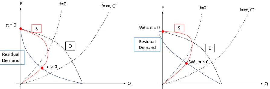
The SFE, introduced by Klemperer and Meyer (1989), is an equilibrium in a game where firms choose their own supply function flexibly. Firms offer their own supply schedule si-multaneously, and the market then clears such that the total supply matches the demand at a certain price. In a model with demand uncertainty, the market clears after the uncer-tainty is realized. The SFE is defined as a (pure strategy) Nash equilibrium in this game. A remarkable feature of the SFE is that it is characterized as the locus of ex post optimal price-quantity pairs given the other firms’ supply functions. The logic is as follows. Each firm guesses the others’ (fixed) supply schedules. After the realization of demand uncertainty, combined with the other firms’ supply functions, a residual demand function is determined. Suppose that a firm chooses its ex post optimal price-quantity pair along with the residual demand. Since the ex post optimal points vary according to the uncertainties realized even
1
though the firm assumes that the others’ supply functions are fixed, the locus of ex post optimal points becomes a function from price to quantity. Since the firm can obtain ex post optimized profit through this supply function, it has no incentive to take other supply functions in the first stage, given others’ supply functions. Thus, the locus is a best response to the others’ supply functions. By considering such best responses for each firm, we obtain Nash Equilibrium in this game, in other words, SFE.
The most famous application of the SFE would be wholesale electricity markets. In dereg-ulated wholesale electricity markets, generating companies offer their own supply schedules and retailers bid to supply their own customers such as consumers or other companies. If there are many retailers, the setting of supply function competition fits well with the struc-ture in those markets because the retail demand is subject to exogenous shocks such as weather, holidays, and major sporting events. SFE has been extensively used as a tool to analyze electricity markets, both theoretically and empirically, ever since Green and Newbery (1992) employed it to analyze wholesale electricity markets.2
Another important, but less focused, interpretation would be the equilibria in the con-jectural variation model with appropriately specified strategies. In general, the conjectural variation first introduced by Bowley (1924) implies that each firm chooses its quantity while believing that other firms change their quantities by rjdqi in response to a change in firmi’s
quantity dqi. It has been used in empirical literature to capture various market structures
in a reduced form.3 A major critique on this model is that it contradicts the equilibrium
concept in the field of economics, that is, firms are not assumed to choose quantity, given others’ quantity.4 However, in supply function competitions, strategies are (usually
posi-2
Vives (2011) introduces uncertainty into the cost function rather than the demand function, treating it as asymmetric information. Holmberg et al. (2013) show that the SFE in step functions, such as actual offers in the electricity markets, converge to a continuous SFE as the steps becomes finer. Since it is difficult to obtain an analytical solution of the SFE, computation methods to calculate it are also developed in the operations research literature (see Holmberg (2009)).
3
Iwata (1974) and Gollop and Roberts (1979) propose empirical methods to estimate or test the conjec-tural variation. They also apply it to Japanese plate glass industry and US coffee industry. Brander and Zhang (1993) estimate the conjectural variation in the US airline industry with dynamic settings. See also Bresnahan (1989) for review and discussion on the conjectural variation.
4
tively sloped) supply functions. Therefore, other firms change their quantity in response to a quantity change by one firm. In other words, at the SFE, the conjectural parameter rj
is determined by the equilibrium strategy of firm j. Of course, there might be countless equilibria if there is no uncertainty in the market because the shape of each supply function only affects the off-equilibrium outcomes and works as an empty threat. However, in the market with demand uncertainty, the SFE restricts the set of possible outcomes much more narrowly and helps us to understand the market.
1.2
Mixed Oligopoly, Partial Privatization, and CSR
In this paper, we introduce (partially) public firms into the SFE.5 Oligopoly markets with
public firms, called mixed oligopolies, were first examined by Merrill and Schneider (1966) and are extensively discussed in the literature.6 Matsumura (1998) generalizes it to the model
of partial privatization by introducing a partially public firm that maximizes a weighted av-erage of its own profit and the social welfare. In mixed oligopoly markets, the effects of the public firms are not straightforward because of strategic interactions.7 For instance, De
Fraja and Delbono (1989) show that welfare may be higher when a public firm is a profit-maximizer rather than a welfare-profit-maximizer, and Matsumura (1998) finds that the optimal level of partial privatization is neither full privatization nor full nationalization. Matsumura and Sunada (2013) examine a mixed oligopoly with misleading advertising competition and find that a public firm engages in rather than cancels out the misleading advertisement. Even if firms are fully symmetric but concerned about social welfare, the economic implica-tion could be completely different from standard models with profit-maximizing firms. For
oligopolistic game,” and Cabral (1995) provides an explicit example of the repeated game of which the CV solution is an exact reduced form of the equilibrium.
5
Mixed oligopolies occur in various industries, such as the airline, steel, automobile, railway, natural gas, electricity, postal service, education, hospital, home loan, and banking industries.
6
See, De Fraja and Delbono (1989), Fjell and Pal (1996), Matsumura and Kanda (2005), and Ghosh and Mitra (2010).
7
instance, Ghosh and Mitra (2014) examine an oligopoly market where every firm maximizes a weighted average of its own profit and social welfare. Competition among firms with so-cial welfare concerns can be understood as that among firms in transition and developing economies, where the extent of private ownership is restricted, or that among firms with CSR. They compare Cournot and Bertrand competition in a symmetrically differentiated market and show that Bertrand competition yields higher profit and lower social welfare than Cournot competition when profit is weighted sufficiently low. Therefore, we must be careful in considering the existence of (partially) public firms. Fortunately, it turns out that in supply function competition, a public firm encourages private firms to take socially better action through strategic complementarities in terms of the slopes of each supply function.
The remainder of the paper is organized as follows. Section 2 presents the general model. Section 3 analyzes the linear-quadratic model. Section 4 concludes the paper. The proofs of propositions can be found in the appendix.
2
The General Model
With symmetric and private firms, Klemperer and Meyer (1989) characterize the SFE under demand uncertainty as solutions of a differential equation and examine some of its general properties. In this subsection, we characterize the SFE with partially public firms anal-ogously and examine the general properties. In the next subsection, we specify a model with a linear demand function and quadratic cost functions in order to further clarify the implication of the effects of the public firm.
Let us denote the demand function as Q=D(p) +ǫ, wherepis the price of the product and ǫ is a scalar random variable with strictly positive density everywhere on the support [ǫ, ¯ǫ]. We assume that −∞ < D′
(p) < 0, and D′′
(p) ≤ 0. The firms have identical cost functions C s.t. C′
(q) ≥ 0 and 0 < C′′
(q) < ∞ ∀q ∈ [0, ∞). Without loss of generality, let C′
(0) = 0.8 A strategy for firm i(i= 1, 2) is defined as a function mapping from price 8
into quantity: Si : [0, p)→(−∞, ∞). Here, we focus on pure strategy Nash equilibria, in
which Si maximizesi’s payoff given that j choosesSj (i, j = 1, 2, j 6=i).
Given Sj,firm i’s ex post objective function is as follows:
vi(p) = (1−θ) [p(D(p, ǫ)−Sj(p))−C(D(p, ǫ)−Sj(p))] (1)
+ θ ˆ pˆ
p
D( ˙p, ǫ)dp˙+pD(p, ǫ)−C(D(p, ǫ)−Sj(p))−C(Sj(p))
.
Therefore, the first order condition is derived as follows:
∂vi
∂p = (1−θ)
(D(p) +ǫ−Sj(p)) + (p−C
′
(D(p) +ǫ−Sj(p))) D
′
(p)−S′
j(p)
(2)
+ θ
(p−C′(D(p) +ǫ−Sj(p)))D
′
(p) + (C′(D(p) +ǫ−Sj(p))−C
′
(Sj(p)))S
′
j(p)
= 0.
SinceSi is determined by the locus of the optimal pricep
∗
(ǫ) and the corresponding quantity
D(p∗
(ǫ)) +ǫ−Sj(p
∗
(ǫ)), we can replace D(p) +ǫ−Sj(p) bySi. Then, the above equation
becomes a differential equation:
S′
j(p) =
(1−θi) [Si+ (p−C
′
(Si))D
′
(p)] +θi[(p−C
′
(Si))D
′
(p)] (1−θi) (p−C′(Si)) +θi[(p−C′(Si))−(p−C′(Sj))] ≡
fi(p, Si, Sj). (3)
Since a set of functions (S1, S2) that solves a system of differential equations Sj′ (p) =
fi(p, Si, Sj) for i = 1,2, j 6= i satisfy the first order condition given the others’
strate-gies, it is an SFE if the payoff function, given the others’ stratestrate-gies, satisfies the second order conditions. In a model with only private firms, it is known that the symmetric SFE strategy S = Si (i = 1, 2) must satisfy 0 < S
′
Proposition 1 (Necessity of positive slope) If ǫ has full support (ǫ=−D(0), ¯ǫ=∞)
and S is symmetric SFE tracing through ex post optimal points, then∀p≥0, S satisfies (3) and 0 < S′
(p)<∞. Furthermore, S is bounded from below by a function S0(p, θ) with its
derivative
S0′
(p) =−Dp(p) +Dpp(p) (p−C
′
(S0(p)))
(1−θ)−Dp(p)C′′(S0(p))
. (4)
Proof. See the appendix.
As can be seen from eq. (4),S0′
(p, θ) is increasing inθfor allp, and thus, the lower bound
S0(p, θ) approaches the (inverse) marginal cost function when θ goes up. It is also worth
noting that, even if θ approaches 1, S0(p, θ) generally does not converge to the (inverse)
marginal cost function, C′−1
(p). Thus, we cannot guarantee that firms behave (almost) in a socially optimal way even if they have social welfare concerns and hardly care about profits. In the following section, we specify the demand and cost functions to analyze the asym-metric SFE and the role of a public firm.
3
Linear Demand and Quadratic Cost Function
We specify the cost functions and a demand function for an analytical solution. The identical cost functions are defined as C(S) = c2S2 and the total demand function is defined as
Q = D(p, ǫ) = α +ǫ−mp. That is, U(Q) = α+ǫ m
Q− 1
mQ
2/2, where U is a surplus
function. Suppose playerj’s strategy to beqj =Sj(p) =a+bp. Then, the residual demand
is written as
Therefore, the ex post profit maximization problem for firm i, given the others’ strategies, is written as follows:
max
p (1−θi) [pqi(p, ǫ)−C(qi(p, ǫ))] (6)
+ θi[U(qi(p, ǫ) +Sj(p))−C(qi(p, ǫ))−C(Sj(p))].
We can consider the ex post optimal price for eachǫby taking the first order condition with respect to p. Since the corresponding qi for each ǫ is determined along the residual demand
function qi(p, ǫ), we can obtain the following locus of optimal points by canceling out ǫ in
the FOC and (5):
qi =
(m+b) +θi(bc−1)b
(1−θi) +c(m+b)
p+ θiabc
(1−θi) +c(m+b)
.
Then, the SFE is constructed from the following supply functions:
Si(p) = a
∗
i +b
∗
ip for all i= 1, 2,
where
a∗i =
θia
∗
jb
∗
jc
(1−θi) +c m+b∗j
, and (7)
b∗i =
m+b∗
j
+θi b
∗
jc−1
b∗
j
(1−θi) +c m+b
∗
j
≡Bi(b
∗
j; θi) (i= 1, 2, j 6=i). (8)
Suppose b∗
j 6= 0. Then, since a
∗
1 = a
∗
2 = 0 must hold to satisfy eq. (7), we can obtain the
SFE by solving eq. (8).
Even though eq. (8) is difficult to solve analytically, we can obtain some properties of the equilibrium without solving it explicitly. If we take b∗
i as a function of b
∗
j, b
∗
i shifts upward
whenθi increases. On the other hand, b
∗
i is increasing inb
∗
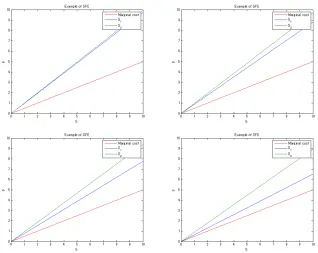
Figure 1: Numerical examples of SFE where m = 1, c = 0.5, and θ2 = 0. θ1 = 0.1: upper
left, θ1 = 0.4: upper right, θ1 = 0.7: lower left, and θ1 = 0.999: lower right
Here, suppose that firm 1 is partially privatized and firm 2 is completely private. If we increase θ1, b
∗
1 shifts upward. Therefore, not only b
∗
1 but also b
∗
2 would increase since b
∗
2 is
increasing in b∗
1. (Numerical examples are illustrated in Fig. 1.)
Proposition 2: (Effect of partial privatization) If we consider a linear demand
func-tion and quadratic cost funcfunc-tions, an SFE is characterized as Si(p) = b
∗
ip ∀i = 1, 2, where
b∗
i =
m+b∗
j
+θi b
∗
jc−1
b∗
j
/
(1−θi) +c m+b
∗
j
(j 6= i). Furthermore, if firm 2 is a private firm (θ2 = 0), then both S1′ (p) and S
′
2(p) increase when θ1 increases.
Proof. See Appendix.
Since both firms’ supply functions become closer to the (inverse) marginal cost function for larger θ1, the social welfare increases withθ1. Thus, we can state the following corollary.
Corollary of Proposition 2: (Mixed oligopoly) Suppose firm 2 is a private firm
Figure 2: Effects on social welfare and profits. (α = 5,m = 1, c= 0.5, E[ǫ] = 0, E[ǫ2] = 2,
and θ2 = 0.)
Thus, existence of a public firm increases social welfare in supply function competition, in contrast to the Cournot competition examined by Matsumura (1998). (Welfare improvement is illustrated in Fig. 2.)
Although we do not have any analytical solutions of eq. (8) for arbitrary θ1 and θ2, we
can solve it for symmetric social concern: θ1 = θ2 = θ. In addition, it turns out that the
[image:11.612.155.449.76.323.2]Proposition 3: (Symmetric SFE in a linear-quadratic model) In a symmetric
setting (θ1 =θ2 =θ), we can obtain the unique symmetric SFE:
Si(p) = −
m+p
m2+ 4m(1−θ)/c)
2 (1−θ) p ∀i= 1,2.
Furthermore, it converges to the (inverse) marginal cost function as θ →1.
Proof. See Appendix.
We can interpret the symmetric θ as the extent of corporate social responsibility and an increase inθ as the improvement in the industry’s social concern. The model guarantees that the supply function shifts upward monotonically as the industry’s social concern improves and that it converges to the socially optimal level as θ→1.
4
Conclusion
References
Bowley, Arthur L., The Mathematical Groundwork of Economics: An Introductory
Trea-tise, Oxford University Press, 1924.
Brander, James A. and Anming Zhang, “Dynamic Oligopoly Behaviour in the Airline
Industry,” International Journal of Industrial Organization, 1993, 11 (3), 407–435.
Bresnahan, Timothy F., “Empirical Studies of Industries with Market Power,” Handbook
of Industrial Organization, 1989, II, 1012–1057.
Cabral, Lu´ıs M.B., “Conjectural Variations as a Reduced Form,”Economics Letters, 1995,
49(4), 397–402.
De Fraja, Giovanni and Flavio Delbono, “Alternative Strategies of a Public Enterprise
in Oligopoly,” Oxford Economic Papers, 1989,41 (2), 302–311.
Farrell, Joseph and Carl Shapiro, “Horizontal Mergers : An Equilibrium Analysis,”
American Economic Review, 1990,80 (1), 107–126.
Fjell, Kenneth and Debashis Pal, “A Mixed Oligopoly in the Presence of Foreign Private
Firms,” The Canadian Journal of Economics, 1996, 29 (3), 737–743.
Ghosh, Arghya and Manipushpak Mitra, “Comparing Bertrand and Cournot in Mixed
Markets,”Economics Letters, 2010,109 (2), 72–74.
and , “Reversal of Bertrand-Cournot Rankings in the Presence of Welfare Concerns,”
Journal of Institutional and Theoretical Economics, 2014, 170(3), 496–519.
Gollop, Frank M. and Mark J. Roberts, “Firm Interdependence in Oligopolistic
Mar-kets,”Journal of Econometrics, 1979,10 (3), 313–331.
Green, Richard J. and David M. Newbery, “Competition in the British Electricity
Holmberg, P¨ar, “Numerical Calculation of an Asymmetric Supply Function Equilibrium with Capacity Constraints,” European Journal of Operational Research, 2009, 199 (1), 285–295.
and David Newbery, “The Supply Function Equilibrium and Its Policy Implications
for Wholesale Electricity Auctions,”Utilities Policy, 2010,18 (4), 209–226.
, , and Daniel Ralph, “Supply Function Equilibria: Step Functions and Continuous
Representations,”Journal of Economic Theory, 2013,148 (4), 1509–1551.
Iwata, Gyoichi, “Measurement of Conjectural Variations in Oligopoly,” Econometrica,
1974,42 (5), 947–966.
Klemperer, Paul D. and Margaret A. Meyer, “Supply Function Equilibria in Oligopoly
under Uncertainty,” Econometrica, 1989,57 (6), 1243–1277.
Matsumura, Toshihiro, “Partial Privatization in Mixed Duopoly,” Journal of Public
Eco-nomics, 1998, 70 (3), 473–483.
and Osamu Kanda, “Mixed Oligopoly at Free Entry Markets,” Journal of Economics,
2005,84 (1), 27–48.
and Takeaki Sunada, “Advertising Competition in a Mixed Oligopoly,” Economics
Letters, 2013, 119(2), 183–185.
Merrill, William C. and Norman Schneider, “Government Firms in Oligopoly
Indus-tries: A Short-Run Analysis,”The Quarterly Journal of Economics, 1966,80(3), 400–412.
Vives, Xavier, “Strategic Supply Function Competition with Private Information,”
Econo-metrica, 2011,79 (6), 1919–1966.
Weyl, E. Glen and Michal Fabinger, “Pass-Through as an Economic Tool: Principles
Appendix
A
Proofs
We characterize the differential equation (3) by the following series of lemmas.
Lemma 1 The locus of points satisfyingf(p, S) = 0is a continuous, differentiable function
S =S0(p), satisfying
(i) S0(0) = 0,
(ii) S0(p)<(C′
)−1(p), ∀p > 0,
(iii) S0′
(p) is positive and increasing in θ,∀p≥0, and
(iv) S0′
(0)< C′′1(0).
Proof of Lemma 1: Differentiating (3) w.r.t. S yields
fS(p, S) =
p−C′
(S) +SC′′
(S) (p−C′
(S))2
so for all ¯p, S¯
6
= (0, 0) such that f p,¯ S¯
= 0,
fS p,¯ S¯
= 1 ¯
p−C′ ¯
S +
¯
S
¯
p−C′ ¯
S
C′′ ¯
S
¯
p−C′ ¯
S
= 1−
1
(1−θ)Dp(¯p)C ′′ ¯
S
¯
p−C′ ¯
S 6= 0.
Therefore, by the implicit function theorem, f(p, S) = 0 implicitly defines, in the neighbor-hood of any such ¯p, S¯
,a unique functionS=S0(p),which is continuous and differentiable.
To prove (i) and (ii), observe that∀θ ∈[0, 1), S0(p) andp−C′
or both zero since −∞< Dp(p)<0 and f(p, S0(p)) = 0. Hence, p > C
′
(S0(p)) whenever
S0(p) > 0. Furthermore, S0(0) = 0 is the unique solution to f(0, S) = 0. For all p > 0,
S0(p)>0 (otherwise, S0(p) = 0 andp−C′
(S0(p))>0) andp > C′
(S0(p)).SinceC′′
>0, we can take the inverse function of C′
and obtain (C′
)−1(p) > S0(p) for all p > 0. Here,
as p → 0, the upper bound of S0(p) converges to zero and S0(p) >0 for all p > 0. Then,
S0(p)→0 as p→0. Thus, S0(p) is continuous atp= 0.
To prove (iii) and (iv), differentiate f(p, S0(p)) = 0 totally with respect to p and
substitute using this equation to get
S0′
(p) =−Dp(p) +Dpp(p) (p−C
′
(S0(p)))
(1−θ)−Dp(p)C′′(S0(p))
.
Now limp→0S0 ′
(p) exists and equals
−(1 Dp(0)
−θ)−Dp(0)C′′(0) ≡
S0′
(p),
where 0< S0′
(p)< C′′1(0),and thus S
0(p) is continuous and differentiable at p= 0. Q.E.D.
Lemma 2 The locus of the points satisfying f(p, S) = ∞ is a continuous, differentiable
function, S =S∞
(p)≡(C′
)−1(p). Hence, S∞
(0) = 0 and 0< S∞′
(p)<∞ ∀p≥0.
Proof of Lemma 2 (same as the proof of claim 2 in KM ): From (3), S∞
(p) solvesf(p, S∞
(p)) =∞implies thatS∞
(p) solvesp−C′
(S∞
(p)) = 0.Hence, sinceC′′
>0,
S∞
(p) = (C′
)−1(p) ∀p. The stated properties of S∞
(p) follow from the assumptions for
C′
(S). Q.E.D.
Proof of Lemma 3 (same as the proof of claim 3 in KM): Since S
p−C′(S) is finite
and increasing in S as long as p > C′
(S), for a given ¯p, f(¯p, S) is finite and monotonically increasing in S for S ∈[0, (C′
)−1(p)). Below the f =∞ locus, 0> S
p−C′(S) >−∞. Hence,
since 0> Dp >−∞, 0> f(p, S)>−∞. Q.E.D.
Lemma 4 If S(p) solves (3) and the other firm takes S(p), the second derivative of i’s payoff with respect topfor a givenǫevaluated at an intersection ofS(p)and residual demand function D(p) +ǫ−S(p) is written as
∂2v
i(p, ǫ; S(p))
∂p2 |p=p∗ = (Dp(p
∗
)−S′
(p∗
)) ((1−θ) +C′′
(D(p∗
) +ǫ−S(p∗
))) (9)
−C′′
(D(p∗
) +ǫ−S(p∗
)) (Dp(p
∗
)−S′
(p∗
))2−(1−θ)S′
(p∗
),
where p∗
is the price that solves D(p∗
) +ǫ−2S(p∗
) = 0.
Proof of Lemma 4: Given that j chooses S(p), the second order derivative of i’s
payoff with respect to p for a given ǫ is
∂2v
i(p, ǫ; S(p))
∂p2 = (2−θ){Dp(p)−S
′
(p)} −C′′
(D(p) +ǫ−S(p)) (Dp(p)−S
′
(p))2
+ (p−C′
(D(p) +ǫ−S(p))) (Dpp(p)−S
′′
(p))
+θS′
(p)−θC′′
(S(p)) (S′
(p))2+θ(p−C′
(S(p)))S′′
(p). (10)
If S(p) solves (3), we can differentiate (3) totally with respect to p to obtain an expression for S′′
(p):
S′′
(p) = X1 ((1−θ) (p−C′
X1 ≡ [(1−θ)S
′
(p) + (1−C′′
(S(p))S′
(p))Dp(p) + (p−C
′
(S(p)))Dpp(p)] [(1−θ) (p−C
′
(S(p)))]
−[(1−θ)S(p) + (p−C′
(S(p)))Dp(p)] [(1−θ) (1−C
′′
(S(p))S′
(p))].
Substituting (3) for S(p) into (11) gives
S′′
(p) = (1−θ)S
′
(p) + (1−C′′
(S(p))S′
(p)) (Dp(p)−(1−θ)S
′
(p)) + (p−C′
(S(p)))Dpp(p)
(1−θ) (p−C′
(S(p))) , (12) and thus, when S(p) solves (3), S′′
(p) in (10) is replaced by (12). Moreover, if we evaluate atp=p∗
wherep∗
solves D(p∗
) +ǫ−2S(p) = 0, (10) becomes (9). Q.E.D.
By these lemmas, we can prove Proposition 1.
Proof of Proposition 1 Satisfaction of (3) ∀p ≥ 0 is a necessary condition for a
supply function defined for allp≥0 to trace through ex post optimal points when the other firm commits to the same supply function. To show that 0 < S′
(p) < ∞ ∀p ≥ 0 is also a necessary condition, we show that if, for some p, S ever crosses either f = 0 from below or
f =∞ from the left, then S must eventually violate the global optimality9.
Once trajectoryScrossesf = 0 from below,S′
become and stays negative and, from (A2),
S′′
also becomes and stays negative. Therefore, the trajectory would eventually intersect the
S = 0 axis at a point (p0, 0) with p0 > C
′
(0), where S′
(p0) = f(p0, 0) = 1−1θDp(p0).
Therefore, for ǫ = e(0, p0), Q = D(p0, ǫ) = 0 by definition and then, residual demand
D(p0, ǫ)−S(p0) = 0. Then, given firmjtakesS,p0satisfies the first order condition but that
results inqi =qj = 0 and SW =πi =vi = 0. On the other hand, since S
′
(p0) = 1−1θDp(p0),
S(p) and the residual demand D(p, ǫ)−S(p) for the same ǫ = e(0, p0) cross each other 9
Figure 3: A supply function (satisfying FOC and symmetry) violating global optimality. (Left: θ = 0, Right: 0< θ <1 )
at another point (p1, q1) where q1 > 0 and p1 > C
′
(q1) (Fig.3). Since SW, πi, vi > 0 at
(p1, q1), firm i has an incentive to adjust from p0 to p1. Thus, S eventually violates the
global optimality. Q.E.D.
Proof of Proposition 2 WLOG, let assume that firm 1 is a partially public firm
(θ1 ∈[0,1]) and firm 2 is a private firm (θ2 = 0). Then, Bi(bj;θi) is rewritten as follows:
B1(b2; θ1) =
(m+b2) +θ1(b2c−1)b2
(1−θ1) +c(m+b2)
,
and
B2(b1)≡B2(b1; 0) =
(m+b1)
1 +c(m+b1)
.
At the equilibrium, b∗
1 and b
∗
2 satisfy the following:
F (b∗
1, b
∗
2; θ)≡
b∗
1−B1(b
∗
2; θ1)
b∗
2−B2(b
∗
1)
= 0
Then, the Jacobian ofF (b∗
1, b
∗
2; θ) w.r.t. (b
∗
1, b
∗
2) is written asJ(b∗
1, b∗2) =
1 −∂B1(b∗2, θ1)
∂b∗
2
−∂B2(b∗1)
∂b∗
1 1
, and then, by Implicit Function Theorem, db∗ 1 dθ1 db∗ 2 dθ1 =−J
−1
b
−dB1(b∗2, θ1)
dθ1 0 = 1
1− ∂B1(b∗2;θ1)
∂b∗
2
∂B2(b∗
1) ∂b∗ 1
1 ∂B1(b∗2;θ1)
∂b∗
2
∂B2(b∗1)
∂b∗ 1 1
∂B1(b∗2;θ1)
∂θ1
0
Then, what we need to show is that ∂B1(b∗2;θ1)
∂θ1 >0,
∂B1(b∗2;θ1)
∂b∗
2 <1, and
∂B2(b∗1)
∂b∗
1 ∈(0,1).
In general, we have
∂Bi(bj;θi)
∂bj
= {1 +θi(2bjc−1)} {(1−θi) +c(m+bj)} −c{(m+bj) +θi(bjc−1)bj}
{(1−θi) +c(m+bj)}2
Thus, for firm 2,
∂B2(b1)
∂b1
= 1
{1 +c(m+b1)}2
>0.
Furthermore, we can rewrite ∂Bi(bj;θi)
∂bj as the following:
∂Bi(bj;θi)
∂bj
= 1 + {−(1−θ)cbj} {1−θi+cm+cbj} −cbj(1−θ)
2
−(1−θi)cmbjc−cm{2−θi+cm}
{(1−θi) +c(m+bj)}2
.
Since the second term is less than 0, we have ∂Bi(bj;θi)
∂bj <1. Lastly, by taking the derivative
w.r.t. θ1,
∂B1(b
∗
2; θ1)
∂θ1
= (1−θ1) (b2c−1)b2+c(m+b2) (b2c−1)b2+ (m+b2) +θ1(b2c−1)b2
{(1−θ1) +c(m+b2)}2
= b
3
2c2+ (b22c2−b2c)m+m
{(1−θ1) +c(m+b2)}2
= b
3
2c2+ b2c− 12
2 m+3
4m
{(1−θ1) +c(m+b2)}2
Thus, if we suppose thatθ2 = 0 , then
db∗
1
dθ1 >0 and
db∗
2
dθ1 >0 Q.E.D.
Proof of Proposition 3 By proposition 1, for S to be a symmetric SFE, S must
satisfy (3) and 0< S′
(p)<∞.In the linear case, (3) is rewritten as follows:
S′(p) = (1−θ)S+{p−C
′
(S)} ·Dp(p)
(1−θ){p−C′
(S)} = (1−θ)S+{p−cS} ·(−m)
(1−θ){p−cS} .
In an autonomous form,
dS
dt = (1−θ)S+{p−cS} ·(−m) dp
dt = (1−θ){p−cS}.
Then, dS dt dp dt =
(1−θ+mc)S−mp
−c(1−θ)S+ (1−θ)p =
(1−θ+mc) −m
−c(1−θ) (1−θ)
S p .
For any eigenvalue r, the following equation must be satisfied:
det
(1−θ+mc) −m
−c(1−θ) (1−θ)
−rI
= 0
⇔r = 2 (1−θ) +mc±
p
m2c2+ 4mc(1−θ)
We have different and unequal eigenvalues. For each eigenvalue r1, r2, the eigenvectors are
defined as follows:
(1−θ+mc) −m
−c(1−θ) (1−θ)
−riI
ui wi
= 0
⇔
((1−θ+mc)−ri)ui−mwi
−c(1−θ)ui+ ((1−θ)−ri)wi
= 0.
Then,
ui
wi
= (1−θ)−ri
c(1−θ)
= (1−θ)−(1−θ)−
mb±√m2c2+4mc(1−θ) 2
c(1−θ)
= −mb∓
p
m2c2+ 4mc(1−θ)
2c(1−θ)
= −m∓
q
m2+ 4m(1−θ)
c
2 (1−θ) .
Let larger eigenvalue be r1. Then, wu11 < 0 and wu22 > 0. Since the eigenvalues are real and
unequal, the solution to the differential equation is written as
S p
=A1e
λ1t
u1 w1 +A2e
λ2t
u2 w2 (13)
where A1 and A2 are arbitrary constants. Here, if A1 6= 0,
S
p =
A1eλ1tu1+A2eλ2tu2
A1eλ1tw1+A2eλ2tw2
= A1u1+A2 e
(λ2−λ1)t u2
A1w1+A2(e(λ2−λ1)t)w2
→ wu1
1
and thus, all trajectories eventually leave the region between f = 0 and f = ∞, and their slope becomes negative. Therefore, the only remaining S that satisfies the necessary conditions is (13) with A1 = 0:
S(p) = −m+
q
m2+4m(1−θ)
c
2 (1−θ) p≡
g(θ)
h(θ). (14)
Suppose that the other firm takes this linear supply function. Then, the local optimality for firm i’s payoff function is satisfied along S(p) by lemma 5, and the residual demand is also linear since the demand function is defined as linear. Since both the residual demand and marginal cost are linear in p, given ǫ, firm i’s profit function πi is written as a function
quadratic inp. On the other hand, since the demand function and industrial marginal costs are linear in p, given ǫ, SW is written as a function quadratic in p. Therefore, the payoff for firm i, which is the weighted average of i’s profit and SW, is written as a quadratic function. Therefore, the local optimal point given ǫ is actually a unique global maximizer given ǫ. Thus, (14) is a symmetric SFE.
We check the effect of θ. Since g(1) =h(1) = 0 by l’Hopital’s Rule we have
lim
θ→1S(p) = limθ→1
g(θ)
h(θ) = limθ→1
g′
(θ)
h′
(θ) = limθ→1
m c
p q
m2+ 4m(1−θ)
c
= p
c
Thus, θ converges to 1 and the supply function converges to the marginal production cost.
![Figure 2: Effects on social welfare and profits. (α = 5, m = 1, c = 0.5, E[ǫ] = 0, E[ǫ2] = 2,and θ2 = 0.)](https://thumb-us.123doks.com/thumbv2/123dok_us/189500.517858/11.612.155.449.76.323/figure-eects-social-welfare-prots-a-e.webp)