D.R.EVOL: Three Dimensional Realistic Evolution

(1)

ABSTRACT

ROBINSON, DOUGLAS MICHAEL. D.R. EVOL: Three Dimensional Realistic Evolution. (Advisor: Jeffrey Thorne)

Simplifying assumptions are necessary to model complex biological processes. Although some assumptions may make sense mathematically, they are often im-plausible when literally translated. This is especially true of the independence among codons assumption, which states that the evolutionary rate at one codon is independent of the evolutionary rate at surrounding codons. Sites within proteins must interact in order to form intricate three-dimensional binding sites and activa-tion domains. This dissertaactiva-tion details the derivaactiva-tion of a procedure for statistical inference when independent change is not assumed.

The procedure is implemented in a Bayesian framework where Markov chain Monte Carlo methods permit approximation of posterior distributions. Analy-ses with the procedure on data sets with two and three taxa are explored and biologically plausible values of the solvent accessibility and pairwise interaction parameters are inferred. Via these analyses, we illustrate the chronological order-ing of amino acid replacements and the detection of specific events to be positively selected. We also find spatial clustering of the amino acid replacements that have most affected sequence-structure compatibility during the evolution of primate eosinophil-derived neurotoxin proteins.

(2)

D.R. EVOL: THREE DIMENSIONAL REALISTIC EVOLUTION

by

Douglas Michael Robinson

A dissertation submitted to the Graduate Faculty of North Carolina State University

in partial fulfillment of the requirements for the Degree of

Doctor of Philosophy BIOINFORMATICS

Raleigh 2003

APPROVED BY:

(3)

DEDICATION

To the loving memory of my mom, Heidi D. Robinson. I will always know that you are proud of me.

(4)

PERSONAL HISTORY

Douglas Robinson was born on April 2, 1973, to Donald and Heidi Robinson, in Newton, Massachusetts. He spent his formative years growing up in Need-ham, Massachusetts, a small suburb located 10 miles southwest of Boston. While growing up, Doug enjoyed the outdoors, especially swimming, skiing, camping and hiking mountains in nearby New Hampshire and Vermont.

After graduating from Needham Highschool in 1991, Doug attended the Uni-versity of Massachusetts at Amherst majoring in mathematics and pre-med. This gave him the opportunity to test his academic wings with both difficult math courses, such as differential and partial differential equations, and challenging sci-ence courses, such as organic chemistry, human anatomy and physiology and ge-netics. His desire to enter medical school led him to spend a tremendous amount of time and money on applications, as well as countless hours studying for the brutal MCAT exam. After receiving politely worded rejection letters from every single medical school to which he applied, thoughts concerning his future quickly changed, and the decision to attend the University of Vermont for graduate work was made.

It was during this time that two events occurred which would change his life forever. First was the release of Austin Powers: International Man of Mystery, in which Doug was introduced to a character known as Dr. Evil. Although the details of Dr. Evil’s life were quite inconsequential, in a twisted sense of irony it seemed rather strange how Dr. Evil’s childhood paralleled Doug’s own: Summers in Rangoon, luge lessons, etc. It was in this vein that Dr. Evil would shape Doug’s thoughts and make him want to major in World Domination. Because this was

(5)

not a recommended graduate level major at UVM, Doug decided to continue along the mathematics route. The second event was meeting his future wife Heather at a Halloween party in October of 1997. Rumor has it that it was not until their third date that they would actually see each others true identity under their respective Halloween costumes. School was a major focus of Doug’s life, but fortunately Heather had a large influence on Doug, by teaching him that there was more to life than just school....and thoughts of world domination, of course.

Doug’s Master’s thesis led him to enter the world of Protein Evolution, and to the understanding of a little band known as Phish. Between acquiring many live recordings of the band, as well as many scientific journal articles on protein evolution, he would decide that his education had to continue. Through the inter-net, Doug found North Carolina State University and a professor named Dr. Jeff Thorne who studied just that. Thus, a short 850 mile journey south and 4 + years later, Doug completed his Ph.D. with the creation of Three Dimensional Realis-tic Evolution, or D.R. EVOL for short. This phylogeneRealis-tic software package may not dominate the entire world, but may at least dominate the world of molecular evolution.

In the future Doug has two goals: First, find as many ways as possible to dominate the world. Besides this, Doug also wants to go into the pharmaceutical industry where he hopes to make powerful drugs that will drive up the cost of health care. The idea being, that hopefully this cost will inadvertently put an enormous amount of pressure and strain on the medical schools to do something about the problem. To complete the vicious circle of life, Doug then dreams of the day when the medical schools contact him for relief, to which he will only sit

(6)

back and laugh in their faces. Then calmly, he will remind them that this situation could have been avoided if they had only accepted his medical school applications when they had the chance so many years ago!!!

(7)

ACKNOWLEDGEMENTS

What a long strange trip its been. This dissertation is the culmination of effort of many people for which I am most grateful. I am especially grateful to my advisor Jeff Thorne who had what appeared to be an unending amount of patience, trust and moral support to guide me through a Ph.D that was enormous in scope. Also, I want to thank him for his immeasurable amount of confidence that I could accomplish such a difficult task. Jeff, I will always appreciate the many hours spent in the intellectual “stratosphere”, discussing the sometimes minute intricacies of the model, especially those where gigantic leaps were made. I would also like to thank the other members of my committee, Bruce Weir, Spencer Muse, Bill Atchley, and Ed Buckler for their helpful comments and support. On a personal note, I want to thank Ed for his in depth insight into the future directions of my project, Spencer for his writing ability and for teaching me how to white water kayak, Bill for his humorous comments to help ease the tension, and Bruce for entrusting me with the Bioinformatics GSA and for allowing me the honor to brew beverages for the Bioinformatics Summer Institute. Besides my committee, none of this would be possible if were not for those who may have not been on my committee, but whose influence and assistance made this initial idea a reality. For instance David Jones and Nick Goldman, but also Hirohisa Kishino, whose statistical ingenuity and infinite generosity made going to, and living in Tokyo Japan an experience that I will remember and treasure for the rest of my life.

I am indebted to my family, especially my brother Chris, his wife Tara, and niece Jordan; for my laws Stephanie France, and Kevin Tyler and my sister

(8)

in-law Heidi Leong for their love and encouragement. I also want to thank my brother in-law Darryl Leong for his cutting sarcasm and for feigning poor golf skills. Don’t worry Darryl, I won’t tell anyone that it was not an act. The most important person however, is my lovely wife Heather. Heather, I could not have done this without your constant love of me during a time when my thoughts and ramblings were incomprehensible. I tried to warn you that it would be difficult, but I think we both learned the hard way that it was more than we bargained for. I promise you that my next dissertation will be on discovering why you ever said yes to me in the first place. I love you!

There are some other family members that I must thank and although they will not be able to read this, I want to thank my two cats, Boobah and Poopoos for their support during this process. By sleeping on the many stacks of papers around my office, they ensured that any sudden wind bursts would not negatively impact my progress. They were also instrumental in reminding me to take time for the truly important tasks, such as the occasional belly-rub and short snack breaks. I am grateful to those in the program of Bioinformatics and Statistical Genetics who put up with my insanity. I will never understand why they listened to me as I rambled on about whatever N.P.R. was discussing during my ride into school. I want to especially thank Debbie Hibbard, whose daily discussions motivated me to get my butt to the gym and work out some of my tension on the rowing machine. Debbie, thanks for always being available to lend an ear to listen to my problems. I also want to thank Dahlia Nielsen for letting me interrupt her work on a regular basis and for being an endless bounty of knowledge.

(9)

wife Heather, Terry Stigers, Stephane Aris-Brosou, Tae-kun Seo, Jeff Thorne, and especially my brother Chris, who patiently endured multiple revisions of my sec-ond manuscript. I also owe it to the Thorne working group namely, Stephane Aris-Brosou, Betsy Scholl, Tae-kun Seo and Jiaye Yu, who spent countless hours listening to me rehearse my presentations. To my many friends at the B.R.C., who I would like to collectively refer to as my answering service, I thank you for taking the time to write those messages and find me, despite my desk being the furthest from the phone. To Jimmy Doi, Errol Strain, Frank Mannino, Betsy Scholl, Stephane Aris-Brosou, David Aylor, Sunil Suchindran, Jack Liu and Josh Starmer, I want to thank you for your friendship and for succeeding to get me out of the office to play frisbee golf, real golf, or just go out to have a drink. You have no idea how much I appreciate your efforts. But I can not forget the person who I consider one of my best friend during this whole process, Andrea Johnson. Your offbeat comments, stories about ponies and almost constant barrages of my theories kept me in check and added a great deal of humor to my life. Andrea, we made it through this and we did it together.

Lastly, I want to thank the band Phish for providing the soundtrack to my dissertation. Through their endless jams, I was able to concentrate on my work and focus in on the many intricacies that my model always seemed to present. I also want to thank the coffee and tea growers around the world for their precious, precious caffeine rich crops. Furthermore, I have to thank the makers of TUMS, or any antacid for that matter, for helping my digestive system cope with the stress. I also want to thank the N.C. State crew team for allowing me valuable time on the rowing machines. This was especially true when I placed second during their

(10)

2000 meter erg time trials. They succeeded in making a 30 year old grad student feel like he could still compete with the undergrads. In conclusion, I want to thank my nephew Brandon Minervini, who at age 7 innocently asked me if the reason I was still in school was if I failed. Well Brandon, I finally passed!

(11)

List of Tables

1.1 The nearly Universal Genetic Code . . . 7

1.2 Time Reversible Nucleotide Models. . . 14

1.3 Codon Models . . . 18

2.1 Priors and Posteriors for the annexin V sequence comparison . . . 68

2.2 Posterior means and 95% credibility intervals for s and p . . . 69

2.3 Priors and Posteriors for the Lysozyme c sequence comparison . . . 74

3.1 Priors and Posteriors for the Lysozyme c sequence comparison . . . 110

3.2 Event placement and measures of positive selection for Lysozyme c . . . 111

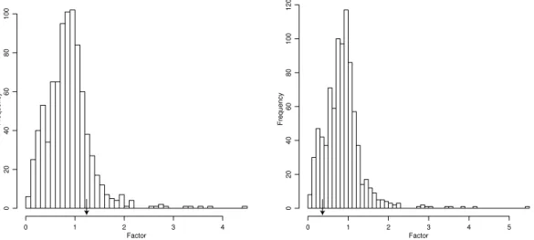
3.3 Priors and Posteriors for the EDN sequence comparison . . . 114

3.4 Event placement and measures of positive selection for EDN protein . . 120-1 3.5 Substitution event site clusters of both positively selected and negatively . 122 3.6 Ancestral node reconstruction of EDN protein . . . 127

3.7 Possible substitution event orders for codons 64 and 132 . . . . 127

(15)

List of Figures

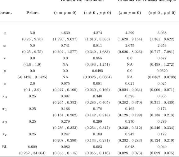
1.1 The four nucleotide bases, Adenine, Guanine, Cytosine and Thymine . . . 5 2.1A Nonsysnonymous rate variation due to structure in mouse annexin V . . . 71 2.1B Comparison for mouse annexin V of effects of solvent accessibility and . . 71 2.2A Nonsysnonymous rate variation due to structure in human lysozyme c . . 72 2.2B Nonsysnonymous rate variation due to structure in Rhesus macaque . . . 72 2.2C Comparison for human lysozyme c of effects of solvent accessibility. . . 75 3.1. Given observed sequences A, B and outgroup sequence O phylogeny . . .106 3.2A. Rate across a randomly sampled path when independence is assumed . . 108 3.2B. Rate across a randomly sampled path when dependence is assumed . . . 108 3.2C. List of codons that interact with codon 61 when site dependencies . . . . 108 3.3. The posterior density of omega for Lysozyme c when site independence .112 3.4. The posterior density of omega for EDN protein when site independence 116 3.5. The values of solvent accessibility and pairwise interactions for ancestral.117 3.6. The values of solvent accessibility and pairwise interactions for accepted.118 3.7. Substitution event site clusters from EDN sequence analysis . . . . 123-4

(16)

Chapter 1 REVIEW

(17)

Introduction

The study of molecular evolution has had a rich history, yet is far from being completely resolved. While a great deal of progress has been made in recent years, there are still many facets that warrant explanation and questions that still need to be answered. With the introduction of high throughput sequencing, genome shot gunning and accelerated PCR methods, it is now possible to obtain massive amounts of high quality sequence data at a rapid pace. With the entire genome of many organisms now complete, in particular the human genome (International Human Genome Sequencing Consortium, 2001, Venter et al. 2001), interest in the field of molecular evolution has seen a dramatic increase. To meet this demand, new and more robust models for comparative sequence analysis and phylogenetic inference are necessary.

The relationship between geneticists and molecular evolutionists is mutually beneficial and cyclical in nature. Geneticists uncover minute components of the process of sequence change using the latest technologies. With this information, molecular evolutionists try to build robust, statistically founded models that dis-cern the relationships between biologically motivated parameters to best fit the model system. Results from these models can then strengthen the support of currently held theories, or discover relationships that were previously unknown. Whatever the circumstance, the relationship between genetics and molecular evolu-tion will provide avenues for future experimentaevolu-tion, as well the means for creating more realistic models and will inevitably broaden our understanding of sequence evolution.

(18)

To begin to model this complex phenomenon, researchers greatly simplify the process of sequence change by making several assumptions and considering only a few biologically realistic factors (Thorne, 2000). Most widely used models of se-quence evolution exploit the assumption that individual sites evolve independently from one another. The independence assumption dictates that a substitution at one site does not influence the rate of substitution at surrounding sites. From a computational standpoint this assumption is quite attractive, for it makes statis-tical inference on evolutionary trees computationally tractable. This calculation is achieved via Felsenstein’s pruning algorithm (Felsenstein, 1981) where the like-lihood of an individual site in an alignment can be easily determined. The full likelihood is subsequently computed simply by taking the product of each individ-ual site likelihood over all sites in the alignment.

The pruning algorithm requires an amount of computation proportional to the sequence length N , the number of internal nodes on the phylogeny (for bifurcating rooted topologies, this equals the number of taxa minus one) and the square of the number of characters states n that are allowed at each site. Typically, models of nucleotide substitution (e.g., Jukes and Cantor, 1969, Kimura, 1980, Felsenstein, 1981, Hasegawa et al., 1985, Felsenstein, 1989) have n = 4, whereas models of amino acid replacement (e.g., Dayhoff et al., 1978, Jones, Taylor and Thornton, 1992b) have n = 20 and models of codon change (e.g., Muse and Gaut, 1994, Gold-man and Yang, 1994) have n = 61. Unfortunately, the computationally attractive assumption of evolutionary independence among sites is not biologically plausible for protein coding sequences. Protein sequences must adopt complex three di-mensional folds and maintain specific activation sites and binding domains. Thus,

(19)

evolution must occur between compatible residues in order to maintain protein functionality. In reality, the effect of a substitution might cascade through the protein, changing the substitution rates at other sites. This is especially true at sites in the protein core because of the densely packed nature of the folded protein structure.

Models are built upon assumptions that may be mathematically reasonable, but are not always considerate of the biological system to which they are applied. Consequently, relaxing certain assumptions may cause results to be computation-ally unobtainable. For instance, to relax the independent evolution among sites assumption, the notion of evolution occurring at individual sites or codons must be extended to the idea of entire sequence evolution. The form of the explicit rate matrix necessary to accomplish this is beyond the capabilities of modern day com-puters. Thus, to calculate likelihoods on phylogenetic trees, alternative methods have to be derived.

The field of molecular evolution is initially presented in a biological context. Without a clear understanding of the biological system under investigation, param-eter estimates and subsequent data analyses have no foundation. A tour through some of the pioneering work that has driven the field of molecular evolution over the past forty years is then presented. Relaxing the independence assumption is a natural step in the long progression of statistical models of evolution and it will be interesting to observe the insights and ramifications that this work will have on the field.

(20)

N _N N N N N _N N N O N N N O N N N O O N N O O Adenine Cytosine Guanine Thymine Uracil

Figure 1.1: The four nucleotide bases, Adenine, Guanine, Cytosine and Thymine, plus the RNA nucleotide Uracil are shown. Adenine and Guanine are purines, while Cytosine, Thymine and Uracil are pyrimidines. Because of the structural similarity, purine-purine or pyrimidine-pyrimidine substitutions are much more likely than substitutions between groups.

Biological Background

The genetic makeup of most organisms is contained within DNA (Deoxyribonu-cleic acid). DNA is composed of four nucleotides: Adenine, Cytosine, Guanine and Thymine, abbreviated A, C, G and T, respectively. The nucleotides come in two varieties, the purines, which includes A and G and the pyrimidines, which in-cludes C and T. All four nucleotides are unique, yet the structural similarity within purines or pyrimidines is substantially higher than that between the two groups (See Figure (1.1)). Just five short decades ago, Watson and Crick, (1953a) pro-posed the structural configuration of the DNA molecule as two antiparallel strands of DNA that combine through hydrogen bonding of nucleotide base pairs. The nat-ural bonding pattern was determined to occur between a purine and a pyrimidine, namely A to T, with the formation of two hydrogen bonds and C to G, through the

(21)

formation of three hydrogen bonds. This arrangement allows a semi-conservative mechanism of DNA replication whereby each parental strand would separate from the unwound double helix and serve as a template for the newly synthesized strand (Watson and Crick, 1953b; Messelson and Stahl, 1958).

DNA is transcribed to RNA (Ribonucleic acid) which is translated to amino acids, the building blocks of proteins. This is known as the central dogma of molecular biology. DNA T ranscription z}|{ ⇒ RNA T ranslation z}|{ ⇒ PROTEIN

DNA and RNA are very similar to one another except for two points. Both DNA and RNA share Adenine, Cytosine and Guanine, but instead of the Thymine base, RNA contains Uracil (U) (See Figure 1). Also, both DNA and RNA bases are each connected to pentose sugar molecules called ribose, but RNA has a hydroxyl group bonded to the 2′ _{carbon of its ribose while DNA has only a single hydrogen}

atom bonded at this position, hence the name de-oxy-ribose.

Three letter combinations of RNA nucleotides code for specific amino acids that are common to all organisms. The sixty-four possible words, or codons, comprise the (nearly) Universal Genetic Code (see Table 1.1). Exceptions to the universal-ity of the genetic code are observed in yeast and certain protozoa, however the most visible is found in mammalian mitochondria. In particular, three noticeable differences include: UGA encoding tryptophan rather than a stop codon; AUA defining methionine instead of isoleucine; and AGA and AGG translating stop codons rather than arginine (e.g., Snustad and Simmons 2000). There are twenty distinct amino acid types in existence, which means that there is some degeneracy

(22)

The Universal Genetic Code

SECOND

U C A G

UUU Phenylalanine UCU Serine UAU Tyrosine UGU Cysteine U U _UUC _{Phenylalanine} _UCC _Serine _UAC _Tyrosine _UGC _Cysteine C

UUA Leucine UCA Serine UAA STOP _UGA STOP A

UUG Leucine UCG Serine UAG STOP _UGG _Tryptophan G CUU Leucine CCU Proline CAU Histidine CGU Arginine U

F

C CUC Leucine CCC Proline CAC Histidine CGC Arginine C

T

I

CUA Leucine CCA Proline CAA Glutamine CGA Arginine A

H

R

CUG Leucine CCG Proline CAG Glutamine CGG Arginine G

I

S

AUU Isoleucine ACU Threonine AAU Asparagine AGU Serine U

R

T

A AUC Isoleucine ACC Threonine AAC Asparagine AGC Serine C

D

AUA Isoleucine ACA Threonine AAA Lysine AGA Arginine A AUG Methionine ACG Threonine AAG Lysine AGG Arginine G GUU Valine GCU Alanine GAU Aspartic Acid GGU Glycine U G _GUC _Valine _GCC _Alanine _GAC _{Aspartic Acid} _GGC _Glycine C GUA Valine GCA Alanine GAA Glutamic Acid GGA Glycine A GUG Valine GCG Alanine GAG Glutamic Acid GGG Glycine G

Table 1.1: The nearly Universal Genetic Code is used to decode all possible three nucleotide combinations into its proper amino acid. The table is set up such that the nucleotide in the left most column corresponds to the first position of the codon, the nucleotide in the top row of the table corresponds to the second position in the codon and the right most nucleotide corresponds to the third position in the codon. Notice the degeneracy of the genetic code as well as the existence of the three stop codons, namely UAA, UAG and UGA, which signal the ribosomes to terminate translation.

in the genetic code. For instance, there are six codons that each translate Leucine, while there are only two codons that translate Histidine. From Table 1.1, one can observe that there are sixty-one sense codons that translate true amino acids and three that translate STOP codons, namely UAA, UAG and UGA. When read, stop codons instruct the ribosomes to terminate the translation process and to sep-arate into their component halves. In most cases, stop or nonsense codons signal the release of a fully translated protein sequence. Yet, in the case of a premature stop codon (i.e. a nonsense mutation), the resultant shortened sequence is most likely non-functional. In these cases, the protein is targeted by the cellular defense

(23)

mechanisms for destruction. Depending on the role of the affected protein in the cell, a nonsense mutation may be lethal.

Each of the twenty amino acids share a common backbone, yet all have unique side chains which emanate from the central carbon atom, denoted Cα. Because

of the composition and arrangement of the atoms within the various side chains, physical and biochemical properties are conferred on each residue. These proper-ties include for example, overall size, polarity, hydrophobicity and charge which have been used by researchers as a basis of comparison (Grantham 1974; Taylor and Jones 1993; Koshi and Goldstein 1995). Because of the common backbone structure, any two amino acids can form a peptide bond. In this reaction, the negatively charged carboxyl terminal of one residue is attracted to the positively charged amino terminal of the next residue. Both are joined via a dehydration synthesis reaction with the expulsion of a single water molecule.

The precise sequence of amino acids is called the primary structure of a protein. Interactions between the side chains of the amino acids cause the linear sequence to contort and adopt unique conformations necessary for the protein to function properly. Changes in the identity of residues in a folded protein may negatively impact surrounding residues, which in a worst case scenario may force a change in the overall structure resulting in a complete loss of function (Purves, Orians and Heller 1992). The fact that any two amino acids can bond complicates the analysis of protein sequences, for in theory an amino acid sequence of length N has 20N

unique possible residue combinations. However, because of negative interactions only a minute fraction of the 20N _{possible sequences ever encode viable proteins.}

(24)

have been classified as local secondary structures. Some examples include α-helices, β-pleated sheets, turns and loops. These secondary structures have been of great interest to molecular evolutionists for it has been proposed that the rate of amino acid replacement depends partly on local secondary structure (Overington et al., 1992; Koshi and Goldstein 1995). The amino acids themselves have differing affini-ties for each of the various secondary structures (e.g., Thorne, Goldman and Jones 1996) and certain amino acids, in particular Proline and Glycine, actually prevent the formation of the α-helix (Purves, Orians and Heller 1992). Secondary struc-tures can stably interact with one another through hydrogen bonds, salt bridges, and Cysteine-Cysteine di-sulfide bonds, forming unique tertiary structures that confer functional specificity to the proteins enabling them to bind other proteins and DNA through the formation of activation and catalytic domains.

One way to describe sites within a folded protein structure is by local secondary structure. Some properties associated with the folded protein are percent solvent accessibility and pairwise interactions with surrounding residues. Given a highly resolved protein crystal structure, these quantities can be defined and fixed for each site in the protein. In general, the percent solvent accessibility is a measure of the degree to which a site is exposed to the surrounding solvent. Intuitively, those residues that lie on the surface of a protein have a large percent accessibility and are generally hydrophilic in nature. Likewise, those sites within the core of the protein have correspondingly low percent accessibility and are filled typically with hydrophobic residues. Hydrophobic residues aggregate similar to the behavior of oil droplets in water. This has led to the proposition that hydrophobicity drives the process of protein folding (Dill, 1990a, Dill, 1990b). In this hypothesis, the

(25)

hydrophobic core of the protein forms first, while the proper folding of the external features of the protein takes place shortly thereafter.

Like gravity, the electrostatic force, or potential between residues within a protein decreases with the square of the three dimensional separation distance. Hence, pairwise interactions can only be defined between those residues that are in close proximity in the folded protein state. Interestingly, residues that are distantly separated along the primary structure of a protein may in fact be located close in three dimensions because of the complex folding pattern of the tertiary structure. In general, proteins are densely packed molecules and sites on the surface of the protein may generally interact with only a few sites, but those in the core inevitably interact with substantially more sites. Amino acid replacements in the core may consequently have greater influence on protein functionality, simply because of their effect on a higher proportion of sites.

It is with this biological background that molecular evolutionists build statis-tical models that try to mimic closely the complex evolutionary substitution pro-cess. Through an enormous amount of trial and error statistical assumptions are relaxed, allowing models to become increasingly more realistic and consequently, more computationally complex in the process. Over the years evolutionary models have themselves evolved to capture these observed behaviors, which is described in the following section.

(26)

Statistical Models

DNA is not a static entity. Over time, all organisms experience mutations in their DNA that have varying effects on the proteins they encode. The reasons for muta-tion events are varied and stem from normal cellular processes to interacmuta-tions with the environment. Some causes include internal sequencing errors in DNA repli-cation, repair mechanisms, insertions and deletions or more severe DNA damage such as the formation of pyrimidine dimers. Unfortunately, the word mutation conjures up images of freakish genetic experiments gone awry and in some cases, mutations can be deleterious to the host. Fortunately, over time these mutations are usually removed from a population through natural selection.

Mutations in which a nucleotide is substituted come in two varieties, namely transitions and transversions. Transitions occur when a nucleotide is replaced by a structurally similar nucleotide, that is Purine → Purine, Pyrimidine → Pyrimidine, while transversions occur when a nucleotide is replaced by a structurally dissimilar nucleotide, that is Purine → Pyrimidine, Pyrimidine → Purine. The ramification of such an event is realized when the codon containing the substituted nucleotide is translated to its corresponding amino acid residue.

Synonymous substitution events do not influence the identity of the encoded amino acid residue in the protein. However, nonsynonymous substitutions cause the translation of a different amino acid residue, yet because of the location of the change, or by possessing similar physical and biochemical properties, the protein may remain fully functional. Whether a substitution is synonymous or nonsynony-mous depends on the identity of the nucleotides that comprise the codon unit at

(27)

the instant of the substitution event. Unlike synonymous substitutions, nonsyn-onymous substitutions are not tolerated equally well across the protein and may be detrimental to overall functionality. In general, researchers have found that the rate of nonsynonymous substitutions on the surface of globular proteins is about twice that of residues buried in the core of the structure (Goldman, Thorne and Jones 1998). In rare instances mutations may impart a selective advantage, allow-ing an organism to better adapt to their surroundallow-ings. These mutations are often passed on to future generations and become fixed in the population.

The effects of nucleotide substitutions can be reflected in the creation of statis-tical models. Most models of molecular evolution rely upon theories of stochastic processes and Markov chains. By definition, a stochastic process is a collection of random variables governed by probabilistic laws defined on a common probability space, while a first order Markov chain is a specific type of stochastic process with the property that the next state of the system depends only on the current value (see Karlin, 1966). In this way, all states of the Markov chain prior to the current value have no influence on the probability of future events.

Nucleotide Models

In 1962, Zuckerkandl and Pauling recognized the fact that DNA sequence infor-mation could be used to classify species. Although at this time, not many se-quences were available for analysis, homologous sese-quences from different species were aligned by hand, and the number of sites that differed were tabulated. This idea was formalized in the theory of parsimony (Edwards and Cavalli-Sforza 1963)

(28)

which, like the notion of Occam’s razor, proposed that the most likely explanation of sequence evolution was the one that minimized the total number of substitution events. In 1965, Zuckerkandl and Pauling proposed the concept of the molecular clock that stated the rate of evolution was constant over time. Consequently, the relationship of any two sequences could then be measured by simply counting the number of differences between them.

Using the statistical theories discussed above, Jukes and Cantor in 1969 altered the field by creating the first stochastic rate matrix, the JC69, which framed molec-ular evolution in the context of a stochastic process. Under this model, the rate of change to any nucleotide is equal to that of any other nucleotide. Consequently, not only is the probability of replacement the same, but the steady state, or lim-iting distribution of the four nucleotides is also equivalent and fixed at 0.25. In general, when building a model of molecular evolution, determining which sequence is ancestral is nearly impossible. For this reason, models are typically constructed with the statistical assumption of time reversibility which makes the ancestral se-quence choice arbitrary. With this assumption, the probability of starting from nucleotide type i and changing to nucleotide type j in a time interval is the same as the probability of starting from j and going backwards to i in the same time duration. The models discussed herein (see Table 1.2) are all time reversible and contain between 1-9 parameters to estimate from the data.

Technological advances increased the availability of DNA sequences and limi-tations of Jukes and Cantor’s JC69 model were more readily apparent. Through greater biological understanding, statisticians and geneticists used the JC69 method-ology as a launch pad for their own models. For instance, researchers noticed that

(29)

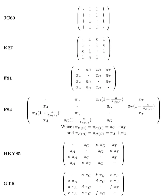
JC69      · 1 1 1 1 · 1 1 1 1 · 1 1 1 1 ·      K2P      · 1 κ 1 1 · 1 κ κ 1 · 1 1 κ 1 ·      F81      · πC πG πT πA · πG πT πA πC · πT πA πC πG ·      F84       · πC πG(1 +πH(G)κ ) πT πA · πG πT(1 + _{πH(T )}κ ) πA(1 +_πH(A)κ ) πC · πT πA πC(1 +_πH(C)κ ) πG ·       Where πH(C) = πH(T )= πC+ πT and πH(A)= πH(G) = πA+ πG HKY85      · πC κ πG πT πA · πG κ πT κ πA πC · πT πA κ πC πG ·      GTR      · a πC b πG c πT a πA · d πG e πT b πA d πC · f πT c πA e πC f πG ·     

Table 1.2: This table lists many of the time reversible models of nucleotide evolution. As one descends the table, the number of free parameters steadily increases from JC69 having one free parameter, to the most general time reversible model, GTR, which has nine free parameters. See the accompanying text for a full description of the models and the various parameters that are incorporated (see also Yang 1997).

(30)

transitions occurred more often than transversions which was incorporated into a model in 1980 called the K2P (Kimura 1980), and subsequently verified with an extensive empirical study (Brown and Simpson 1982). The K2P model is identi-cal to the JC69 except for a new parameter κ, the transition / transversion rate parameter, which affords researchers the ability to estimate how much more likely transitions are in their dataset.

Shortly thereafter, Felsenstein proposed a pair of stochastic models, commonly referred to as the F81 (Felsenstein, 1981), and the F84 (see Felsenstein, 1989). Contradictory to the uniform steady state distribution hypothesized previously (Jukes and Cantor, 1969) Felsenstein recognized that in most cases there exists a nucleotide base composition bias in DNA sequence data. To alleviate this re-striction three degrees of freedom were added to the F81 model by allowing the relative frequency of the nucleotides to vary. The instantaneous rate in this model is proportional to πj, the relative frequency of nucleotide type j. Frequently, good

estimates of the relative frequencies of the four nucleotides are easily derived from counts of the individual nucleotides in the dataset under investigation and used for the remainder of the likelihood calculation. It is reassuring to note that under the independence assumption, the estimates derived by this counting method are very similar to those obtained by estimation through likelihood procedures. The F84 model is an integral part of the evolutionary procedure presented in later chapters of this work, and thus will not be discussed now.

The idea of combining a model that allows the relative frequency of the nu-cleotides to vary with a transition-transversion rate parameter resulted in the for-mation of two models, namely the HKY85 (Hasegawa, Kishino and Yano, 1985)

(31)

and what is commonly referred to as the F84 (Felsenstein, 1989). Only minute differences in how each measures a transition substitution distinguish these mod-els. Similar to the K2P model of Kimura (1980), the HKY85 model captures this behavior using the transition-transversion rate parameter κ. However, the F84 model uses: κπj πH(j) where πH(j)=      πA+ πG if j is a purine πC + πT if j is a pyrimidine (1.1)

which allows the rate of a change for transitions to be conditional on nucleotide group membership. The parameters in both models are estimated through maxi-mum likelihood techniques.

The most general time reversible model contains at most nine parameters to estimate from the data; three for the relative nucleotide frequencies and up to six for each possible pairwise nucleotide substitutions. For this reason it is referred to as the General Time Reversible (GTR) model (e.g., Tavar´e 1986; Yang 1994a; Zharkikh 1994). In order to obtain reasonable estimates for the large number of parameters considered, this model should not be used to analyze datasets with only a few, relatively short sequences. Thus for a particular dataset, in order to choose the optimal model two thoughts must be considered. Adding parameters the model makes it more general and increase its applicability. On the other hand, although more biologically realistic assumptions can be considered, the computa-tional complexity of a model increases with extra parameters. This increases the error variance associated with each parameter estimate (e.g., Zharkikh, 1994). Us-ing too simplified a model may also lead to biased results (e.g., Huelsenbeck, 1995;

(32)

Huelsenbeck and Rannala, 1997). The real trick then, is to strike the perfect bal-ance between incorporating many of the rules that govern the process of evolution, yet still remain general enough to provide wide applicability and provide useful statistical inference without a tremendous increase in computational complexity.

Codon Models

Whether a substitution is synonymous or nonsynonymous depends on the iden-tity of the nucleotides that comprise the codon unit. Underlying the process of nucleotide substitution is the nearly Universal Genetic Code (See Table 1.1), thus the process of nucleotide substitution in coding regions is inherently not inde-pendent among sites. By incorporating the dependence structure of the Genetic Code, models can be built to separate the biases in substitution patterns found at the nucleotide level, from selective constraints found at the amino acid level (e.g., Goldman and Yang 1994; Yang, Nielsen, and Hasegawa 1998).

The codon models that are frequently used are modifications of those originally proposed by Muse and Gaut (1994) and the Goldman and Yang (1994) (see Ta-ble 1.3). The explicit form of both matrices are quite sparse, for each disallows instantaneous changes at more than one codon position, as well as change to pre-mature stop codons. In these Markov models the state space increases to 61 x 61 for the 61 sense codons of the universal genetic code. To model the evolution between two aligned codons that differ in more than one position, both models behave as though there are multiple distinct substitution events that evolve the codon in the given amount of time.

(33)

(a) Muse and Gaut, 1994 Qx,y =      πβ χ If event is synonymous πβ φ If event is nonsynonymous

0 If codons differ at more than one posisiton

(b) Goldman and Yang, 1994

Qx,y =     

u πc(y) κ e−d(aax,aay)/V If codons differ by a transition

u πc(y) e−d(aax,aay)/V If codons differ by a transversion

0 If codons differ at more than one posisiton

(c) Goldman and Yang, 1994 (Simplified)

Qx,y =               

u πc(y) If event is a synonymous transversion

u πc(y) κ If event is a synonymous transition

u πc(y) ω If event is a nonsynonymous transversion

u πc(y) κ ω If event is a nonsynonymous transition

0 If codons differ at more than one position

Table 1.3: Models of codon evolution. The Muse and Gaut codon model (1.3a) uses only 5 parameters. The dual parameterization of the parameter-rich Goldman and Yang codon rate matrix is also given in 1.3b,c. Most of the parameters in 1.3b,c are stationary codon frequencies. Explanation of the parameters used in each model are given in the accompanying text.

The Muse and Gaut model (Table 1.3(a)) accounts for the constraint at the nu-cleotide level through πβ, the equilibrium frequency of the substituted nucleotide

type in the target codon accounting for stop codons. At the amino acid level, this model allows for heterogeneity of rates between synonymous and nonsynonymous substitutions through χ, the synonymous rate parameter and φ, the nonsynony-mous rate parameter. This model has only five rate parameters which can be easily resolved from the data through maximum likelihood procedures.

To model the selective constraints at the nucleotide level, instead of using the equilibrium frequency of the target nucleotide as above, the equilibrium frequency of the target codon, denoted πc(y), can also be used (Goldman and Yang 1994).

(34)

estimates of the codon frequencies, πc(y) is usually derived from the product of the

equilibrium frequencies of the three nucleotides that comprise the codon. These frequencies are then normalized to account for the relative frequency of the three stop codons. Like the K2P (Kimura, 1980) and the HKY85 (Hasegawa, Kishino and Yano, 1985) models of nucleotide substitution, this model also includes the parameter κ, to account for the observance that transitions occur more often than transversions (e.g., Brown and Simpson, 1982).

The Goldman and Yang and Muse and Gaut models of codon substitution can be written to account for differences at the amino acid level using an amino acid distance matrix (Grantham, 1974) (see Table 1.3(b) for the Goldman and Yang parameterization). The Grantham matrix was derived by comparing physical and biochemical properties of the twenty amino acids such as volume, charge, and hydrophobicity. These values are denoted Daax,aay, where aax denotes the amino acid that is translated by codon x in the model, and range from as small as 5 for (ILE - LEU) and as high as 210 for (CYS - PHE). The parameter V is a tuning parameter to allow the distance matrix to better fit the data. A rate normalization constant u is inserted to make the relationQy=61y=1 πc(y)Qy,y = 1, possible (see Table

1.3(b)).

Through experimentation, Goldman and Yang found that this parameteriza-tion did not fit actual data very well, and a simplificaparameteriza-tion involving the assumpparameteriza-tion of uniform distance between all amino acid pairs was imposed. This allowed the complex exponential term to be replaced by the single nonsynonymous / synony-mous rate parameter ω (see Table 1.3(c)). Unlike the Muse and Gaut model, the Goldman and Yang model has 63 parameters to estimate from the data; sixty of

(35)

which are the codon equilibrium frequencies. Lately, these methods have been ex-panded upon to incorporate the behavior seen in lentiviral evolution (Pedersen et al. 1998). This expanded model accounts for the disparity in relative frequencies of the four nucleotides at each of the three codon positions as well as selection against the CpG dinucleotide within codons.

Amino Acid Models

The nucleotide and codon models discussed are all parametric in nature, whereby various parameters are used to define relationships among pairs of nucleotides or codons. When considering models of amino acid evolution, the usual parameters used such as the transition / transversion rate parameter κ, or the nonsynony-mous / synonynonsynony-mous rate parameter ω, lose meaning. Hence, many researchers have instead focused on empirical approaches (Dayhoff et al. 1978; Jones et al. 1992; Gonnet, 1992; Hennikoff and Hennikoff, 1992). Empirical models require a reference data set which, if small, will not provide a good fit to a given data set under investigation (Li`o and Goldman, 1998). However, the advantage to us-ing empirically derived matrices is that they may more realistically capture the unequal transition probabilities among amino acid pairs as seen in true proteins.

Because of the degeneracy of the genetic code, a synonymous substitution may be the result of several substitutions at the nucleotide level. For example, the codons AGU and UCC may differ at all three codon positions, yet when translated, both code for the same amino acid, Serine (see Table 1.1). When analyzing highly diverged sequences, models of amino acid replacement may be beneficial for they

(36)

act as a filter for the noise of multiple substitutions at the DNA level (e.g., Goldman and Yang 1994).

An important method for handling protein evolution was that of Dayhoff, Schwartz and Orcutt in 1978 (see also Dayhoff et al. 1972). In this landmark work, highly similar sets of protein sequences were aligned by hand and subse-quent counts of observed amino acid replacements were tabulated. The small genetic distance between the sequences allowed the assumption of multiple sub-stitutions at a given site to be negligible. With these counts, the Point Accepted Mutation (PAM) matrix was derived. Because the counts came from global align-ments of several protein sequences, the PAM matrix determines the probability for an amino acid replacement located in an average site within an average protein. Unfortunately, the definition of an average site within an average protein becomes difficult to verbalize with any precision, yet despite this apparent drawback, the Dayhoff method has gained wide acceptance and has been used successfully in making phylogenetic inference.

The Dayhoff method was duplicated on a more modern database using a sub-stantially higher amount of sequence information to create the JTT amino acid substitution matrix (Jones, Taylor and Thornton, 1992b). The increase amount of data allowed a more robust estimate of the probability of change between rare amino acid pairs (e.g., Methionine vs. Tryptophan), which were nonexistent in the dataset used for the creation of the PAM matrices. Because very similar methodologies were employed to create the Dayhoff model, the JTT model suffers the same unavoidable consequence of also being defined for an average site in an average protein.

(37)

Through matrix multiplication, Dayhoff et al. (1978) were able to create amino acid transition matrices for various PAM distances. In particular, the commonly used PAM120 and PAM250 matrices were derived by multiplying the PAM matrix by itself 120 and 250 times, respectively, where larger numbers represent greater evolutionary distances. By decomposing the Dayhoff instantaneous rate matrix, the probability of change between amino acid residues can also be calculated for any amount of evolution T using standard matrix exponentiation procedures (e.g., Swofford et al. 1986, Kishino, Miyata and Hasegawa, 1990). This type of model also allowed phylogenetic inference using maximum likelihood, but for some un-known reason it has not enjoyed the same widespread use.

Lastly, instead of working with a large amino acid replacement matrix, re-searchers were able to represent all twenty residues by considering only a finite set of the most conserved physical and chemical characteristics (Koshi, Mindell and Goldstein 1997, 1999; Koshi and Goldstein 1998; Halpern and Bruno 1998). Con-sidering these quantities as fixed, transition matrices based on functions of these properties were then derived. This significantly reduced the number of parameters in the model that may have allowed for accurate parameter estimation, yet may have also oversimplified the true complexities of the evolutionary process, giving results that are often difficult to interpret.

Models That Consider Protein Structure

Starting from a linear sequence of amino acids, the precise manner in which the sequence attains its resultant three dimensional structure is still unknown.

(38)

Fortu-nately, there exist methods to discern the precise structures of proteins. In fact, as of January 1, 2003, the Brookhaven Data Bank (PDB) (Bernstein et al. 1977) contained the three dimensional coordinates of roughly 20,000 proteins. These co-ordinates were mainly derived from protein X-ray crystallography, but were also derived from nuclear magnetic resonance (NMR) techniques. Through precise protein conformations, functionality is conferred. Thus, any disruption in protein structure may easily render the protein non-functional. For example, enzymes are proteins that possess a high degree of specificity and function to catalyze precisely one reaction, which is why they are commonly referred to as lock-and-key proteins. For this reason, although it has long been observed that divergence in homologous protein sequences occurs rapidly, the corresponding change in their associated pro-tein structure is much less severe because of the strong selective pressure to main-tain functionality (e.g., Chothia and Lesk 1986; Flores et al. 1993; Russell et al. 1997).

One way in which researchers could explore the ramifications of amino acid replacements in proteins is with site-directed mutagenesis. However, using this method would not only be slow and tedious, but would inevitably be unsuccessful at testing the vast amount of amino acid replacement combinations. It was later hypothesized that by using the database of known sequences one could compile lists of protein characteristics in various local site environments to discern what properties had been conserved through evolutionary time (Koshi and Goldstein 1995). In order to maintain the overall conformation of the protein, it has been observed that amino acids that share physical and biochemical attributes tend to replace one another more often on average than those that are more disparate

(39)

(e.g., Zuckerkandl and Pauling, 1965; Dayhoff et al. 1978; Parisi and Echave, 2001). Others have defined an explicit distance between amino acid residues based on measures of hydrophobicity, charge and side chain volume (e.g., Grantham, 1974; Taylor and Jones, 1993). Yet, it is not clear whether the forces behind evolutionary change are governed by these properties.

The idea that the rate of amino acid replacement depends on local secondary structure is not novel (Overington et al. 1992; Koshi and Goldstein, 1995). Fur-thermore, many researchers have understood the importance of incorporating struc-tural and functional information into models to improve evolutionary and phylo-genetic inference (e.g., Koshi and Goldstein, 1995, 1997; Thorne, Goldman and Jones 1996; Goldman, Thorne and Jones, 1998). Yet, exactly how each group has achieved this goal has been quite varied. However, researchers have been able to use large databases to analyze the relationships between amino acid residues and secondary structural elements with solved tertiary protein structures. For instance, researchers have analyzed the databases of aligned sequences to create amino acid transition matrices (Dayhoff et al. 1978, Jones et al. 1992). Unfortunately in these cases, only a single matrix was produced to explain the evolutionary history of all sites within a sequence regardless of the local environment of that site. Building on this idea, the structural databases were later analyzed to construct transition matrices for various secondary structural environments and surface accessibilities (Koshi and Goldstein, 1995, 1997; Goldman, Thorne and Jones 1998; Thorne et al. 1996). The results of Thorne et al. (1996) mainly showed that hydrophobicity was highly conserved, that the volume of a residue was slightly conserved in core re-gions because of tight internal packing constraints and surprisingly, that secondary

(40)

structural elements were less conserved. Similar to the problems faced by the PAM and JTT matrices, Koshi and Goldstein (1998) problematically note that within each environment, amino acids are treated uniformly by the given matrix.

Logically following this idea even further, one may desire site-specific amino acid transition matrices. In order to obtain reasonable parameter estimates how-ever, the tremendous amount of data necessary for their creation make this too daunting a task (Li`o and Goldman, 1998). One way to handle this is to assume that sites can be classified in a limited number of structural classes with which one can create specific transition matrices by analyzing large databases of sequences (Thorne, Goldman and Jones, 1996; Goldman, Thorne and Jones, 1998; Li`o et al. 1998). However, in most cases it may be unreasonable to assume that only a finite number of structural classes can accurately account for the vast diversity of sites found in proteins and their associated structures.

One way to simplify the study of proteins is to classify individual sites into categories based on location (internal vs. external), on local secondary structures (α− helix, β− sheet, loop, etc.), and percent solvent accessibility. Using various property combinations, large tables have been compiled to analyze the replacement patterns observed in aligned sequences (Overington et al., 1990, L¨uthy et al., 1991, Topham et al., 1993, Wako and Blundell, 1994). Because these tables were derived regardless of evolutionary considerations, applications of such matrices to answer phylogenetic questions becomes difficult. Another way to simplify matters is to consider codon position and chemical properties of the amino acids themselves such as charge, acidity and hydrophobicity as surrogates for experimentally determined protein structures (Naylor and Brown, 1997). Because of the low number and type

(41)

of structures analyzed, the applicability of their method to the broader range of globular proteins would most certainly be diminished.

Protein Threading and Pseudo–Energy Potentials

A different approach to discovering sequence structure correlations is through pro-tein threading. The idea is to evaluate the fit of a sequence to a known propro-tein structure based on what is seen in a structural database. There are many meth-ods to evaluate sequence structure fit, but some of the more successful are based on Boltzmann physics. This theory often arises when discussing the energetics of compatibility of protein sequences and related protein structures. In the past Boltzmann physics has been used to describe the energetics of protein conforma-tions (MacArthur and Thornton, 1991, Serrano et al. 1992), with the existence of internal cavities (Rashin et al. 1986), of ion pairs (Bryant and Lawrence, 1991), or with amino acid location preferences (Miller et al. 1987, Koshi and Goldstein, 1998, Koshi et al. 1997, 1999).

The components and exact form of the true forces that stabilize protein struc-ture may never be known explicitly. One approach to calculate protein stability is to determine the Gibbs free energy associated with a true protein. However, these methods typically require intense computations that may explain the inter-est in faster approximation strategies. Creating pseudo-energy potentials is one way to approximate Gibbs free energy, and it has been successfully applied to pro-tein threading. For instance, Jones, Taylor and Thornton (1992b) created a set of pseudo-energy potentials using the Inverse Boltzmann Principle (IBP) as well as

(42)

the Thermodynamic Hypothesis (Anfinsen, 1973). The Thermodynamic Hypothe-sis postulates that the native conformation of a particular protein sequence is that which gives the lowest energy. As it is applied here, the IBP allows the approxi-mation of the energy associated with solvation and pairwise interactions based on the frequency of occurrence in a database. Combined, these relations assume that if a certain conformation is more frequent, it must therefore be stable and thus will be given a low energy. Furthermore, by evaluating the fit of a particular sequence on all known conformations, the most likely native state is then assumed to be the one that gives the lowest energy (Jones, Taylor and Thornton, 1992b).

The potentials derived using the IBP are commonly referred to as knowledge-based potentials of mean force because they contain the information from the diverse assortment of crystal structures from which they were derived. Instead of an exact measure of protein stability, using the IBP determines a measure of how likely a sequence adopts the given fold based on how similar the interactions compare to those most often observed in the structural database of real proteins (Jones and Thornton 1996). To avoid introducing anomalies into the training set, the rarely crystallized non-globular transmembrane proteins, as well as those proteins with unusual prosthetic groups were excluded (Hendlich et al., 1990).

More data often translates to parameter estimates with lower variance. In this vein, the addition of unique crystal structures to the training set should increase the ability of a model to distinguish incorrect conformations from the true native state of the protein as well (Hendlich et al., 1990). Unfortunately, the true forces that stabilize protein structures are not known. Hence, even with an arbitrarily large database there is no guarantee that the calculated energies converge to the true

(43)

stabilization forces of interaction. For a more complete discussion of the drawbacks of empirical energy potentials along with a test on a hypothetical lattice model protein see Thomas and Dill (1996a, 1996b).

One way in which researchers characterize sites within a protein structure is through measures of solvent accessibility. Because X-ray crystallography is some-times a tedious and unsuccessful endeavor, many have focused their efforts on pre-dicting solvent accessibility measures for sites in proteins whose structures have not been determined (e.g., Pascarella et al. 1998; Pollastri et al. 2002; Rost and Sander 1994; Thompson and Goldstein 1996, 1997). However, if the structure of one sequence in a dataset is known, a direct measure of solvent accessibility for each site can be found using the Dictionary of Secondary Structure of Proteins (DSSP) program (Kabsch and Sander, 1983). Assuming that alignment columns contain structurally homologous positions, the solvent accessibility measure can then be extrapolated across taxa.

To obtain the percent solvation for each site the raw solvation value from DSSP must be normalized using the associated amino acid’s relative maximum accessi-bility. The maximum value for each residue is estimated using a fully extended pentapeptide GG(X)GG as the reference state mimics the configuration for which the residue attains its highest accessibility in a folded protein (see Appendix A) (Jones, Taylor and Thornton, 1992b). The normalized values are then subdivided into five solvation categories ranging from very low values representing sites that are completely buried in the protein core, to high values representing sites that are fully exposed (David Jones, personal communication). The cutoff values for each solvation category, γs, are given in Appendix B.

(44)

Within a protein crystal structure, the solvation category of each site is auto-matically fixed. When evaluating the fit of an non-native sequence to a structure, often times the amino acid residue at a site is not equivalent to the reference residue. Because of differences in side chain volume the exact percent solvation is likely to be slightly different than the given value. Because the solvation categories span an interval however, it seems reasonable to assume that the actual solvent accessibility value of the threaded residue will be contained in the given interval.

When examining protein structures, certain substructures, such as α−helices and β−pleated sheets, are common occurrences even within diverse protein folds. Their high frequency corresponds to highly stable energy values as calculated us-ing the IBP. If protein structure is considered in terms of pairwise inter-atomic distances, one can encompass all aspects of secondary structure as favorable inter-actions between pairs of amino acid residues that lie in close proximity in folded proteins. Several methods accomplish this by defining pairwise interactions among amino acids using pseudo–energy potentials (e.g., Hendlich et al., 1990, Jones, Tay-lor and Thornton, 1992b, Kocher et al., 1994, Miyazawa and Jernigan, 1996, Park et al., 1997). However, Sippl (1990) was the first to derive energy potentials for the interactions of all amino acid residue pairs as a function of interatomic Euclidean distance.

By analyzing the set of highly resolved, non-homologous protein crystal struc-tures in the PDB database, counts of all possible amino acid residue pairwise interactions were tabulated (Jones, Taylor and Thornton, 1992b). In their proce-dure, two residues are defined to interact if their Cβ carbon atoms are within 10

(45)

have a true Cβ atom, a fictitious Cβ atom can be constructed using the spatial

geometry of the other atoms in its backbone (David Jones personal communica-tion). The Jones pairwise potentials were derived for five atom pairs, namely, the Cβ ⇒ Cβ, Cβ ⇒ N, Cβ ⇒ O, O ⇒ Cβ, N ⇒ Cβ.

The behavior of the pairwise energy potential is like that of gravitational force. If two residues lie in close proximity, there is only one potential defined for their interaction. The Nitrogen terminus has a slight positive charge, while the Carboxyl end has a slight negative charge, giving the overall residue an electrostatic gradient (N+ _{⇒ COOH}−_{). Because of this polarity, instead of making symmetric counts}

(Dayhoff et al. 1978) only observed counts between two residues if the initial residue fell prior to the second in the order along the protein chain were tabulated (Sippl, 1990). The equation used to derive all pairwise energy potentials used in GenTHREADER (Jones, 1999) is derived in nice detail in Hendlich et al. (1990). The resultant counts for each atom pair are subdivided into three main cate-gories according to their sequence separation along the protein chain. Short range interactions are those for which amino acids are separated by less than 12 residues along the chain and account for some secondary conformations such as α - he-lix formation. Medium range interactions are those for which amino acids are separated by between 12 and 22 residues, and account for substructures such as amphipathic helices and β - sheet motifs. Finally, long range interactions are those for which amino acid residue separation is greater than 22 residues, and account for the overall tertiary structure interaction and final protein conformation (Jones, Taylor and Thornton, 1992b). Although separated by substantial distances along the protein chain, long range interactions do occur, because of residues lying in

(46)

close proximity in the final complex protein conformation.

Conclusion

The history given in the introduction chronicles the state of molecular evolution for protein coding genes as the topic itself has evolved over the years. The models considered assume independence among sites or codons, which is unfortunately not biologically plausible. In order to maintain functionality of the folded protein state, residues must interact. Relaxing the independence assumption comes with a tremendous increase in computation which in the not so distant past would have been intractable. Recently, computer processor speed and advances in Bayesian statistical modelling, such as Markov chain Monte Carlo methods, have increased to the point where such models can now be contemplated. The following chap-ters detail the derivation and implementation of one such model, whose general framework may have broad applicability in the field of molecular evolution.

(47)

References

Anfinsen, C.B.(1973) Principles that govern the folding of protein chains.

Sci-ence 181(96):223-30

Bernstein, F.C., T.F. Koetzle, G.J.B. Williams, E.F. Meyer, Jr., M.D. Brice, J.R. Rodgers, O. Kennard, T. Simanouchi, M. Tasumi (1977) The protein data bank: A computer based archival file macromolecular structures. J. Mol. Biol. 112:535-542

Brown, G.G., and M.V. Simpson (1982) Novel features of animal mtDNA evolution as shown by sequences of two rat cytochrome oxidase subunit II gnes. Proc. Natl. Acad. Sci. 79:3246-3250

Bryant, S.H., and C.E. Lawrence (1991) The frequency of ion pair sub-structures in proteins in quantitatively related to electrostatic potential: A statistical model for nonbonded interactions. Proteins 9:108-119

Chothia, C. and A.M. Lesk (1986) The relation between the divergence of sequence and structure in proteins. EMBO J. 5:823-826

Dayhoff, M.O., R.M. Schwartz, and B.C. Orcutt. (1978) A model of Evolutionary Changes in Proteins. Pp. 345-352 in Atlas of Protein Sequence

and Structure vol. 5, Suppl. 3. National Biomedical Research Foundation, Washington, D.C.

(48)

Dill, K.A.(1990a) Dominant forces in protein folding. Biochemistry 29(31):7133-7155

Dill, K.A. (1990b) The meaning of hydrophobicity. Science 250(4978):297-298

Edwards, A.W.F., and L.L. Cavalli-Sforza (1963) The reconstruction of evolution. Annals of Human Genetics 27:105-106

Felsenstein, J. (1981) Evolutionary trees from DNA sequences: a maximum likelihood approach. J. Mol. Evol. 17, 368 - 376

Felsenstein, J. (1989) Phylogenetic Inference Package (PHYLIP), version 3.2. University of Washington, Seattle. Cladistics 5:164-166

Flores, T.P., C.A. Orengo, D.S. Moss, and J.M. Thornton(1993) Com-parison of conformational characteristics in structurally similar protein pairs.

Protein Sci. 2:1811-1826

Goldman, N., J.L. Thorne, and D.T. Jones(1996) Using evolutionary trees in protein secondary structure prediction and other comparative sequence anal-yses. J. Mol. Biol. 263:196-208

Goldman, N., J.L. Thorne, and D.T. Jones (1998) Assessing the impact of secondary structure and solvent accessibility on protein evolution. Genetics 149:445-458

Goldman, N., and Z. Yang. (1994) A codon-based model of nucleotide substi-tution for protein-coding DNA sequences. Mol.Biol.Evol. 11(5):725-736

(49)

Gonnet, G.H., M.A. Cohen, and S.A. Benner (1992) Exhaustive matching of the entire protein sequence database. Science 256:1443-1445

Grantham, R. (1974) Amino acid difference formula to help explain protein evolution. Science 185:862-864

Hasegawa, M., H. Kishino and T. Yano (1985) Dating of the human - ape splitting by a molecular clock of mitochondrial DNA. J. Mol. Evol. 21, 160 -174

Hendlich, M., P. Lackner, S. Weitckus, H. Floeckner, R. Froschauer, K. Gottsbacher, G. Casari, and M.J. Sippl(1990) Identification of na-tive protein folds amongst a large number of incorrect models. J. Mol. Biol. 216:167-180

Henikoff S., and J.G. Henikoff(1992) Amino acid substitution matrices from protein blocks. PNAS USA. 8, 10915 - 10919

Huelsenbeck, J.P.(1995) Performance of phylogenetic methods in sumulations.

Syst. Biol. 44(1):17-48

Huelsenbeck, J.P., and B. Rannala (1997) Phylogenetic methods come of age: Testing hypotheses in an evolutionary context. Science 276:227-231

International Human Genome Sequencing Consortium(2001) Initial se-quencing and analysis of the human genome. Nature 409:860-921

(50)

Jones, D.T.(1999) GenTHREADER: An efficient and reliable protein fold recog-nition method for genomic sequences. J. Mol. Biol. 287:797-815

Jones DT, Taylor WR, Thornton JM. (1992a) The rapid generation of mutation data matrices from protein sequences. Comput Appl Biosci. Jun; 8(3):275-82

Jones, D.T., W.R. Taylor, and J.M. Thornton (1992b) A new approach to protein fold recognition. Nature 358:86-89

Jones, D.T., and J.M. Thornton(1996) Potential energy functions for thread-ing. Curr. Opin. Struct. Biol. 6:210-216

Jukes, T.H., and Cantor, C.R.(1969) Evolution of protein molecules.

Mam-malian protein metabolism. (Munro, H.N., ed Pp. 21 - 32 Academic Press, New York,

Kabsch, W., and C. Sander(1983) Dictionary of protein secondary structure: pattern recognition of hydrogen - bonded and geometrical features.

Biopoly-mers 22(12):2577-2637

Karlin, S. A first course on stochastic processes. Academic Press, New York: 1966

Kimura, M. (1980) A simple method for estimating evolutionary rate of base substitution through comparative studies of nucleotide sequences. J. Mol.