Graph-Based Unsupervised Learning of Word Similarities Using
Heterogeneous Feature Types
Avneesh Saluja∗
Carnegie Mellon University
Jiˇr´ı Navr´atil
IBM Research
Abstract
In this work, we propose a graph-based approach to computing similarities between words in an unsupervised manner, and take ad-vantage of heterogeneous feature types in the process. The approach is based on the creation of two separate graphs, one for words and one for features of different types (alignment-based, orthographic, etc.). The graphs are con-nected through edges that link nodes in the feature graph to nodes in the word graph, the edge weights representing the importance of a particular feature for a particular word. High quality graphs are learned during training, and the proposed method outperforms experimen-tal baselines.
1 Introduction
Data-driven approaches in natural language process-ing (NLP) have resulted in a marked improvement in a variety of NLP tasks, from machine translation to part-of-speech tagging. Such methods however, are generally only as good as the quality of the data itself. This issue becomes highlighted when there is a mismatch in domain between training and test data, in that the number of out-of-vocabulary (OOV) words increases, resulting in problems for language modeling, machine translation, and other tasks. An approach that specifically replaces OOV words with their synonyms from a restricted vocabulary (i.e., the words already contained in the training data) could alleviate this OOV word problem.
∗
This work was done during the first author’s internship at the IBM T.J. Watson Research Center, Yorktown Heights, NY in 2012.
Vast ontologies that capture semantic similarities between words, also known asWordNets, have been carefully created and compiled by linguists for dif-ferent languages. A WordNet-based solution could be implemented to fill the gaps when an OOV word is encountered, but this approach is not scalable in that it requires significant human effort for a num-ber of languages in which the WordNet is limited or does not exist. Thus, a practical solution to this problem should ideally require as little human su-pervision and involvement as possible.
Additionally, words can be similar to each other due to a variety of reasons. For example, the similar-ity between the wordsoptimize andoptimal can be captured via the high orthographical similarity be-tween the words. However, relying too much on a single feature type may result in false positives, e.g., suggestions of antonyms instead of synonyms. Valu-able information can be gleaned from a variety of feature types, both monolingual and bilingual. Thus, any potential solution to an unsupervised or mildly supervised word similarity algorithm should be able to take into accountheterogeneousfeature types and combine them in a globally effective manner when yielding the final solution.
In this work, we present a graph-based approach to impute word similarities in an unsupervised man-ner and takes into account heterogeneous features. The key idea is to maintain two graphs, one for words and one for the all the features of different types, and attempt to promote concurrence between the two graphs in an effort to find a final solution. The similarity graphs learned during training are generally of high quality, and the testing approach proposed outperforms the chosen baselines.
2 Approach
The eventual goal is to compute the most similar word to a given OOV word from a restricted, pre-existing vocabulary. We propose a graph-based so-lution for this problem, relying on undirected graphs to represent words and features as well as the simi-larities between them. The solution can be broadly divided into two distinct sub-problems, the training and testing components.
2.1 Learning the Graph
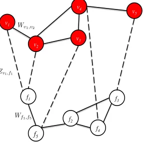
The intuition of our approach is best expressed through a small example problem. Figure 1 shows an example graph of words (shaded) and features (unshaded). For exposition, letv1 =optimize,v2=
optimal, andv3 =ideal, whilef1 =orth |opti, i.e.,
an orthographic feature corresponding to the sub-string “opti” at the beginning of a word, andf5 =
align id´eal, i.e., a bilingual feature corresponding to the alignment of the word “optimal” to the French word “id´eal” in the training data1.
v1
v3
v2
v4
v5
f1
f2
f5
f3
f4
Zv1,f1
Wf1,f5
[image:2.612.115.258.348.490.2]Wv1,v2
Figure 1: An example graph for explanatory purposes. The
nodes in red constitute the word graph, and the nodes in white the feature graph.
There are three types of edges in this scenario. Edges between word nodes (e.g.,Wv1,v2) represent
word similarities, and edges between features (e.g.,
Wf1,f5) represent feature similarities. Edges
be-tween words and features (e.g., Zv1,f1, the dashed
lines) represent pertinent or active features for a given word when computing its similarity with other words, with the edge weight reflecting the degree of importance.
We restrict the values of all similarities to be be-tween 0 and 1, as negative-valued edges in
undi-1such word alignments can be extracted through standard
word alignment algorithms applied to a parallel corpus in two different languages.
rected graphs are significantly more complicated and would make subsequent computations more in-tricate. In an ideal situation, the similarity matrices that represent the word and feature graphs should be positive semi-definite, which provides a nice prob-abilistic interpretation due to connections to covari-ance matrices of multivariate distributions, but this constraint is not enforced here. Future work will focus on improved optimization techniques that re-spect the positive semi-definiteness constraint.
2.1.1 Objective Function
To learn the graph, the following objective func-tion is minimized:
Ω(WV,WF,Z) =α0
X
fp,fq∈F
(Wfp,fq−W
∗
fp,fq)
2 (1)
+α1
X
vi∈V
X
fp∈F
(Zvi,fp−Z
∗
vi,fp)
2
(2)
+α2
X
vi,vj∈V
X
fp,fq∈F
Zvi,fpZvj,fq(Wvi,vj−Wfp,fq)
2
(3)
+α3
X
vi,vj∈V
X
fp,fq∈F
Wvi,vjWfp,fq(Zvi,fp−Zvj,fq)
2
(4)
whereWfp,fq is the current similarity between
fea-ture fp and feature fq (with corresponding initial
value Wf∗p,fq), Wvi,vj is the current similarity
be-tween word vi and word vj, Zvi,fp is the current
importance weight of feature fp for wordvi (with
corresponding initial valueZv∗
i,fp), andα0toα3are
parameters (that sum to 1) which represent the im-portance of a given term in the objective function.
The intuition of the objective function is straight-forward. The first two terms correspond to minimiz-ing the`2-norm between the initial and current
val-ues ofWfp,fq andZvi,fp (for further details on
ini-tialization, see Section 2.1.2). The intuition behind the third term is to minimize the difference between the word similarity of wordsvi andvj and the
fea-ture similarity of feafea-turesfp andfqin proportion to
how important those features are for wordsviandvj
graphs, which in turn ensures smoothness over the two graphs.
The basic idea of minimizing two quantities of the graph in proportion to their link strength has been used before, for example (but not limited to) graph-based semi-supervised learning and label propaga-tion (Zhu et al., 2003) where the concept is applied to node labels (as opposed to edge weights as pre-sented in this work). In such methods, the idea is to ensure that the function varies smoothly over the graph (Zhou et al., 2004), i.e., to promote parame-ter concurrencewithina graph, whereas we promote parameter concurrence across two graphs. In that sense, theαparameters as control the trade-off be-tween respecting initial values vs. achieving consis-tency between the two graphs.
While not necessary, we decided to tie the param-eters together, such thatα0andα2(representing
fea-ture similarity preference for initial values vs. pref-erence for consistency) sum to 0.5, andα1 and α3
sum to 0.5 as well, implicitly giving equal weight to feature similarities and importance weights. In the future, a more appropriate method of learning these
αparameters will be explored.
2.1.2 Initialization
In many unsupervised algorithms, e.g., EM, the initialization of parameters is of paramount impor-tance, as these initial values guide the algorithm in its attempt to minimize a proposed objective func-tion. In our problem, initial estimates for word simi-larities do not exist (otherwise the problem would be considerably easier!). Instead, word similarities are seeded from the initial feature similarities and initial importance weights, and all three quantities are then iteratively refined.
The initial importance weight values are com-puted from the co-occurrence statistics between words and features, by taking the geometric mean of the conditional probabilities (feature given word and word given feature) in both directions:Z∗
vi,fp=
p
P(vi|fp)P(fp|vi). For the initial feature
similar-ity values, the pointwise mutual information (PMI) vector for each feature is first computed, by taking the log ratio of the joint probability with each word to the marginal probabilities of the feature and the word (also done through the co-occurrence statis-tics). Subsequently, the initial similarity is then computed as the normalized dot product between feature vectors: kPMIPMIfp·PMIfq
fpkkPMIfqk.
After computing the initial feature similarity and weights matrices, we remove features that are densely connected in the feature similarity graph by trimming high entropy features (normalizing edge weights and treating the resulting values as a prob-ability distribution). This pruning was done in or-der to speed up the optimization procedure, and we found that results were not affected by pruning away the top one percentile of features sorted by entropy.
2.1.3 Optimization
The objective function (Equations 1 to 4) is con-vex and differentiable with respect to the individ-ual variablesWvi,vj, Wfp,fq, andZvi,fp. Hence, one
way to minimize it is to evaluate the derivatives of the objective function with respect to these variables, set to 0 and solve. The final update equations are provided in the Appendix.
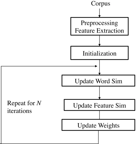
The entire training pipeline is captured in Figure 2. We first compute the word similarities from the initial feature similarities and importance weights, and then update those values in turn, based on the alternating minimization method (Csisz´ar and Tusn´ady, 1984). The process is repeated till con-vergence.
Preprocessing Feature Extraction
Initialization
Update Word Sim Corpus
Update Feature Sim Repeat for N
iterations
[image:3.612.313.543.408.649.2]Update Weights
2.2 Link Prediction
Given a learned word similarity graph (along with a learned feature similarity graph and the edges be-tween the two graphs) and an OOV word with as-sociated features, the proposed solution should also generate a list of synonyms. In a graph-based set-ting, this is analogous to the link prediction prob-lem: given a graph and a new node that needs to be embedded in the graph, which links, or edges, do we add between the new node and all the existing ones? We experimented with two different approaches for link prediction. The first computes word sim-ilarities in the same manner as in training, as per Equation 5. However, since the learned importance weights Zvi,fp (or Zvj,fq) are specific to a given
word, importance weights for the OOV word are ini-tialized in the same manner as in Section 2.1.2 for the words in the training data. Thus, for a given OOV word, we obtain word similarities with all words in the vocabulary through Equation 5, and output the most similar words by this metric.
The second method is based on a random walk approach, similar to (Kok and Brockett, 2010), wherein a probabilistic interpretation is imposed on the graphs by row-normalizing all of the matrices involved (word similarity, feature similarity, and im-portance weights), implying that the transition prob-ability, say from node vi to vj, is proportional to
the similarity between the two nodes. For this ap-proach, only the active features for a given OOV word, i.e., the features that have at least one non-zero Z edge between the feature and a word, are used (see Section 2.3 for more details on active and inactive features). First, M random walks are ini-tialized from each active feature node, each walk of maximum lengthT. For every walk, the number of steps needed to hit a word node in the word simi-larity graph for the first time is recorded. After av-eraging across the M runs, we need to average the hitting times across all of the active features, which is done by weighting the hitting times of each ac-tive featuref∗byP
viZvi,f∗, i.e., the sum across all
rows of a given feature (represented by a column) in the importance weights matrix.
The random walk-based approach introduces three new parameters: M, the number of random walks per active feature, T, the maximum length of each random walk, andβ, a parameter that con-trols how often a random walk should take a Z
edge (thereby transitioning from one graph to the
other) or aW edge (thereby staying within the same graph). If a node has bothZ andW edges, thenβ
is the parameter for a simple Bernoulli distribution that samples whether to take one type of edge or the other; if the node has only one type of edge, then the walk traverses only that type.
2.3 Sparsification
There is a crucial point regarding Equations 1 to 4, namely that restricting the inputted values to be-tween 0 and 1 does not guarantee that the resulting similarity or weight value will also be between 0 and 1, due to the difference in terms in the numerator of the equations. In order to bypass this problem, a projection step is employed subsequent to an up-date, wherein the value obtained is projected into the correct part of then-dimensional Euclidean space, namely the positive orthant. Although slightly more involved in the multidimensional case, i.e., where
n > 1, since the partial derivatives as computed in Equations 5 to 7 are with respect to a single ele-ment, orthant projection in the unidimensional case amounts to nothing more than setting the value to 0 if it is less than 0. This effectively sparsifies the re-sulting matrix, and is similar to the soft-thresholding effect that comes about due to `1-norm
regulariza-tion. Further exploration of this link is left to future work.
However, the sparsification of the graphs/matrices is problematic for the random walk-based approach, in that an OOV word may consist of features that are allinactive, i.e., none of the features have a non-zero
Z edge to the word similarity graph. In this case, we cannot compute which words in our vocabulary are similar to the OOV word. One method to allevi-ate this drawback is to add backZ edges that were removed during training with their initial weights. Yet, we found that adding back all of the features for a test word was worse than filtering out the fea-tures with the highest entropy (i.e., with the most edges to other features) out of the features to add back. The latter approach was thus adopted and is the setup used in Section 3.5.
3 Experiments & Results
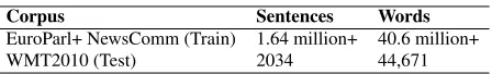
Corpus Sentences Words
EuroParl+ NewsComm (Train) 1.64 million+ 40.6 million+
[image:5.612.76.300.55.89.2]WMT2010 (Test) 2034 44,671
Table 1:Corpus statistics for the datasets used in evaluation.
3.1 Dataset
Table 1 summarizes the statistics of the training and test sets used. We used the standard WMT 2010 evaluation dataset, and the training data consists of a combination of European Parliament and news com-mentary bitext, while the test set is from the news domain. Note that a parallel corpus is not needed as only the English side is used. While the current ex-periment is restricted to English, any language can be used in principle.
3.2 Features
During the feature extraction phase, we first filtered the 30 most common words from the corpus and do not extract features for those words. However, these common words are still used when extracting distri-butional features. The following features are used:
• Orthographic: all substrings of length 3, 4, and 5 for a given word are extracted. For exam-ple, the feature “orth |opt”, corresponding to the substring “opt” at the beginning of a word, would be extracted from the word “optimal”.
• Distributional (a.k.a., contextual): for a given word, we extract the word immediately preced-ing and succeedpreced-ing it as well as words within a window of 5. These features are extracted from a corpus without the 30 most common words filtered. An example of such a feature is “LR the+cost”, representing an instance of a preceding and succeeding word for “optimal”, extracted from the phrase “the optimal cost”. Lastly, all distributional features that occur less than 5 times are removed.
• Part-of-Speech (POS): for example, “pos JJ” is a POS feature extracted for the word “optimal”.
• Alignment (a.k.a., bilingual): alignment fea-tures are extracted from alignment matrices across languages. For every word, we filter all words in the target language (treating En-glish, our working language, as the source) that have a lexical probability less than half the
maximum lexical probability, and use the re-sulting aligned words as features. For exam-ple, “align id´eal” would be a feature for the word “optimal”, since the French word “id´eal” is aligned (with high probability) to the word “optimal”. Note that the assumption during test time is that alignment features are not available for OOV words; if they were, then the word would not be OOV. Nonetheless, alignment in-formation can be utilized indirectly in the link prediction stage from random walk traversals of in-vocabulary nodes.
Statistics on the number of features broken down by type are presented in Table 2, for 3 different vocab-ulary sizes. In the experiments, we concentrated on the 10,000 and 50,000 size vocabularies.
3.3 Baselines
When selecting the baselines, we had two goals in mind. Firstly, we wanted to compare the proposed approach against simpler alternatives for generating word similarities. The baselines were also chosen so as to correspond in some way to the various fea-ture types, since a main advantage of our approach is that it effectively combines various feature types to yield global word similarity scores. This choice of baselines also provides insight into the impact of the various feature types chosen; the idea is that a baseline corresponding to a particular feature type would be indicative of word similarity performance using just that type. Three baselines were initially selected:
• Distributional: a PMI vector is computed for each word over the various distributional fea-tures. The inner product of two PMI vectors is computed to evaluate the similarity of two words. We found that this baseline performed poorly relative to the other ones, and thus de-cided not to include it in the final evaluation.
• Orthographic: based on a simple edit distance-based approach, where all words within an edit distance of 25% of the length of the test word are retrieved.
Vocabulary Words Features Alignment Distributional Orthographic POS
Full 93,011 780,357 325,940 206,253 248,114 50 50k-vocab 50,000 569,890 222,701 204,266 142,873 50 10k-vocab 10,000 301,555 61,792 199,256 40,457 50
Table 2:Statistics on the number of features extracted based on the number of words, broken down by feature type. Note that the distributional features are only those with count 5 and above.
words (as per the lexical probabilities in the matrices) are extracted.
3.4 Evaluation
Automatic evaluation of an algorithm that computes similarities between words is tricky. The judgment on whether two words are synonyms is still done best by a human, requiring significant manual effort. Therefore, during the experimentation and parame-ter selection process we developed an inparame-termediate form of evaluation wherein a human annotator as-sisted in creating a pseudo “ground truth”. Prior to creating the ground truth, all OOV words in the test set were identified (i.e., no match in our vocabulary), resulting in 978 OOV words. Named entities were then manually filtered, resulting in a final test set of 312 words for evaluation purposes.
To create the ground truth, we generated for each test OOV word a set of possible synonyms using the alignment and orthographic baselines, as per Section 3.3. Naturally, many of the words generated were not legitimate synonyms; human evaluators thus re-moved all words that were not synonyms or near synonyms, ignoring mild grammatical inconsisten-cies, like singular vs. plural. Generally, a synonym was considered valid if substituting the word with the synonym preserved meaning in a sentence.
The final evaluation was performed by a human evaluator. The two baselines and the proposed ap-proach generated the top three synonym candidates for a given OOV test word and both 1-best and 3-best results were evaluated (as in Table 3). Final performance was evaluated using precision and re-call. Recall is defined as the percentage of words for which at least one synonym was generated, and precision evaluates the number of correct synonyms from the ones generated.
3.5 Results
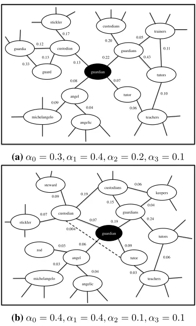
Figure 3 looks at the neighborhood of words around the word “guardian”. Note that while only two dif-ferent α parameter configurations are compared in
Test Word Synonym 1 Synonym 2 Synonym 3
pubescent puberty adolescence nanotubes sportswoman sportswomen athlete draftswoman
briny salty saline salinity
Table 3: Example of the annotation task. The suggested
syn-onyms are real output from our algorithm.
the figure, we investigated a variety of settings and found thatα0 = 0.3, α1 = 0.4, α2 = 0.2, α3 = 0.1
worked best from a final evaluation perspective. The first point to note is that the graph in Fig-ure 3b is generally more dense than that of FigFig-ure
guardian custodian
angel
guardians
tutor 0.13
0.22
0.08 0.07
guard guardia
stickler
0.17
0.13 0.12
custodians
trainers
tutors
0.20 0.05
0.43
michelangelo
angelic 0.09
0.04
teachers 0.06 0.33
0.10 0.11
(a)α0= 0.3, α1= 0.4, α2= 0.2, α3= 0.1
guardian
custodian
angel
guardians
tutor 0.07 0.19
0.06 0.09 steward
stickler 0.09
0.07
custodians
keepers
tutors 0.15
0.04
0.24
michelangelo
angelic 0.03
0.04
teachers 0.03
0.06 0.19
0.06
rod 0.03
0.004
[image:6.612.331.529.348.677.2](b)α0= 0.4, α1= 0.4, α2= 0.1, α3= 0.1
1 2 3 4 5 0
1 2 3 4 5 6 7 8 9
10x 10
5
Number of Elements
Iteration
10k Word Similarity
HHLL HLLH LHHL NHNL
(a)Word similarity matrix sparsity
0 1 2 3 4 5
0 5 10 15x 10
5
Number of Elements
Iteration 10k Weights
HHLL HLLH LHHL NHNL
[image:7.612.336.520.56.123.2](b)Weights matrix sparsity
Figure 4: Word similarity and weights matrices sparsities for 10,000-word vocabulary.
3a. For example, Figure 3b contains an edge be-tween “custodian” and “custodians”, whereas Figure 3a does not. In the latter graph, there is a higher pref-erence for smoothness over the graph and thus the idea is that “custodian” and “custodians” are linked via the smooth transition “custodian”→“guardian”
→“guardians”→“custodians”, whereas in the for-mer, there is a higher preference to respect the ini-tial values, which generates this additional edge. We also observed weak edges between words like “cus-todian” and “tutor” in Figure 3b but not in Figure 3a. The effect of the parameters on the sparsity of the graph is definitely apparent, but generally the learned graphs are of high quality. A further anal-ysis reveals that for many of the words in the cor-pus, the highest weighted features are usually align-ment features; their heavy use allows the algorithm to produce interesting synonym candidates, and em-phasizes the importance of bilingual features.
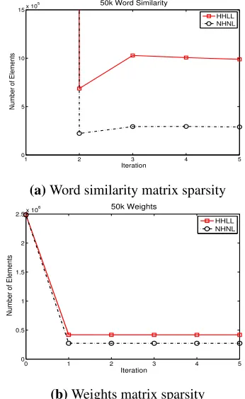
To underscore the point regarding impact of pa-rameters on graph sparsity, Figures 4 and 5 present the number of elements in the resulting word sim-ilarity and weights matrices (graphs) vs. iteration for vocabulary sizes of 10,000 and 50,000
respec-Configuration α0 α1 α2 α3
[image:7.612.104.273.57.342.2]HHLL 0.4 0.4 0.1 0.1 NHNL 0.3 0.4 0.2 0.1 HLLH 0.4 0.1 0.1 0.4 LHHL 0.1 0.4 0.4 0.1
Table 4: Legend for the charts in Figures 4 and 5. H
corre-sponds to “high”, L to “low”, and N to “neutral”.
1 2 3 4 5
0 5 10
15x 10
5
Number of Elements
Iteration
50k Word Similarity
HHLL NHNL
(a)Word similarity matrix sparsity
0 1 2 3 4 5
0 0.5 1 1.5 2 2.5x 10
6
Number of Elements
Iteration 50k Weights
HHLL NHNL
(b)Weights matrix sparsity
Figure 5: Word similarity and weights matrices sparsities for 50,000-word vocabulary.
tively, with Table 4 providing a legend to the curves in those figures. Higherα weights for terms 1 and 2 in the objective function result in less sparse solu-tions. The density of the matrices also drops drasti-cally after a few iterations and stabilizes thereafter.
Lastly, Tables 5 and 6 present the final results of the evaluation, as assessed by a human evaluator, on the 312 OOV words in the test set. While the re-sults on the 1-best front are marginally better than the edit distance-based baseline, 3-best the perfor-mance of our approach is comfortably better than the baselines. Testing was done with the word similarity update method.
[image:7.612.340.513.172.454.2]Method Precision Recall F-1
[image:8.612.85.290.56.111.2]τ matrix 31.1% 67.0% 42.5% orthographic 37.5% 92.3% 53.3% 50k-nhnl 37.2% 100% 54.2%
Table 5: 1-best evaluation results on WMT 2010 OOV words
trained on a 50,000-word vocabulary. Our best approach (“50k-nhnl”) is bolded
Method Precision Recall F-1
τ matrix 96.7% 67.0% 79.1% orthographic 89.9% 92.3% 91.1% 50k-nhnl 92.6% 100% 96.2%
Table 6: 3-best evaluation results on WMT 2010 OOV words
trained on a 50,000-word vocabulary. Our best approach (“50k-nhnl”) is bolded
prediction approach was sub-optimal for several rea-sons. Firstly, it was difficult to use the learned im-portance weights as is, since the resulting weights matrix was so sparse that many test words simply did not have active features. This issue resulted in the vanilla variant of the random walk approach to have very low recall. Therefore, we adopted a “mixed weights” strategy, where we selectively in-troduced a number of features previously inactive for a test word, not including the features that had high entropy. Yet in this case, the random walks get stuck traversing certain edges, and a good sampling of similar words was not properly achievable.
A general issue that arose during link prediction is that the orthographic features tend to dominate the candidate synonyms list since alignment features are not utilized. If instead we assume that align-ment features are accessible during testing, then the random walk-based approaches do marginally better than the word similarity update method, but further investigation is warranted before drawing any defini-tive conclusions.
4 Related Work
We used the objective function and basic formula-tion of (Muthukrishnan et al., 2011), but corrected their derivation of the optimization and introduced methods to handle the resulting complications. In addition, (Muthukrishnan et al., 2011) implemented their approach on just one feature type and with far fewer nodes, since their word similarity graph was actually over documents and their feature similar-ity graph was over words. Recently, an
alterna-tive graph-based approach for the same problem was presented in (Minkov and Cohen, 2012). However, in addition to requiring a dependency parse of the corpus, the emphasis of that work is more on the testing side. Indeed, we can incorporate some of the ideas presented in that work to improve our link pre-diction during query time. The label propagation-based approaches of (Tamura et al., 2012; Razmara et al., 2013), wherein “seed distributions” are ex-tracted from bilingual corpora and are propagated around a similarity graph, can also be easily inte-grated into our approach as a downstream method specific to machine translation.
Another approach to handle OOVs, particularly in the translation domain, is (Zhang et al., 2005), wherein the authors leveraged the web as an ex-panded corpus for OOV mining. If web access is un-available however, then this method would not work. The general problem of combining multiple views of similarity (i.e., across different feature types) can also be tackled through multiple kernel learn-ing (MKL) (Bach et al., 2004). However, most of the work in this field has been on supervised MKL, whereas we required an unsupervised approach.
An area that has seen a recent resurgence in popu-larity is deep learning, especially in its applications to continuous embeddings. Embeddings of word distributions have been explored in (Mnih and Hin-ton, 2007; Turian et al., 2010; Weston et al., 2008).
Lastly, while not directly relevant to our work, the idea of using a graph-based framework to combine both monolingual and bilingual features was also presented in (Das and Petrov, 2011).
5 Conclusion & Future Work
In this work, we presented a graph-based approach to computing word similarities, based on dual word and feature similarity graphs, and the edges that go between the graphs, representing importance weights. We introduced an objective function that promotes parameter concurrence between the two graphs, and minimized this function with a simple alternating minimization-based approach. The re-sulting optimization recovers high quality word sim-ilarity graphs, primarily due to the bilingual features, and improves over the baselines during the link pre-diction stage.
semi-definiteness constraints. Other link prediction tech-niques should be explored, as the current techtech-niques have pitfalls. Richer features that model more re-fined aspects can be introduced. In particular, fea-tures from a dependency parse of the data would be very useful in this situation.
References
Francis R. Bach, Gert R. G. Lanckriet, and Michael I. Jordan. 2004. Multiple kernel learning, conic duality,
and the smo algorithm. InProceedings of the
twenty-first international conference on Machine learning, ICML ’04.
I. Csisz´ar and G. Tusn´ady. 1984. Information
geome-try and alternating minimization procedures. Statistics
and Decisions, Supplement Issue 1:205–237.
Dipanjan Das and Slav Petrov. 2011. Unsupervised part-of-speech tagging with bilingual graph-based
projec-tions. InProceedings of the 49th Annual Meeting of
the Association for Computational Linguistics: Hu-man Language Technologies - Volume 1, HLT ’11, pages 600–609.
Stanley Kok and Chris Brockett. 2010. Hitting the right
paraphrases in good time. InHuman Language
Tech-nologies: The 2010 Annual Conference of the North American Chapter of the Association for Computa-tional Linguistics, HLT ’10, pages 145–153.
Einat Minkov and William W. Cohen. 2012. Graph
based similarity measures for synonym extraction
from parsed text. In TextGraphs-7: Graph-based
Methods for Natural Language Processing.
Andriy Mnih and Geoffrey Hinton. 2007. Three new graphical models for statistical language modelling. In
Proceedings of the 24th international conference on Machine learning, ICML ’07, pages 641–648.
Pradeep Muthukrishnan, Dragomir R. Radev, and
Qiaozhu Mei. 2011. Simultaneous similarity learning and feature-weight learning for document clustering. In TextGraphs-6: Graph-based Methods for Natural Language Processing, pages 42–50.
Majid Razmara, Maryam Siahbani, Gholamreza Haffari, and Anoop Sarkar. 2013. Graph propagation for para-phrasing out-of-vocabulary words in statistical
ma-chine translation. In Proceedings of the 51st Annual
Meeting of the Association for Computational
Linguis-tics, ACL ’13.
Akihiro Tamura, Taro Watanabe, and Eiichiro Sumita. 2012. Bilingual lexicon extraction from comparable
corpora using label propagation. InProceedings of the
2012 Joint Conference on Empirical Methods in Natu-ral Language Processing and Computational NatuNatu-ral
Language Learning, EMNLP-CoNLL ’12, pages 24– 36, Stroudsburg, PA, USA. Association for Computa-tional Linguistics.
Joseph Turian, Lev Ratinov, and Yoshua Bengio. 2010. Word representations: a simple and general method for
semi-supervised learning. InProceedings of the 48th
Annual Meeting of the Association for Computational Linguistics, ACL ’10, pages 384–394.
Jason Weston, Fr´ed´eric Ratle, and Ronan Collobert. 2008. Deep learning via semi-supervised embedding.
InICML, pages 1168–1175.
Ying Zhang, Fei Huang, and Stephan Vogel. 2005. Min-ing translations of oov terms from the web through
cross-lingual query expansion. InProceedings of the
28th annual international ACM SIGIR conference on Research and development in information retrieval, SIGIR ’05, pages 669–670.
Dengyong Zhou, Olivier Bousquet, Thomas Navin Lal, Jason Weston, and Bernhard Sch¨olkopf. 2004. Learn-ing with local and global consistency. In Sebastian Thrun, Lawrence Saul, and Bernhard Sch¨olkopf,
edi-tors,Advances in Neural Information Processing
Sys-tems 16. MIT Press, Cambridge, MA.
Xiaojin Zhu, Z. Ghahramani, and John Lafferty. 2003. Semi-supervised learning using gaussian fields and
harmonic functions. In Proceedings of the
Twenti-eth International Conference on Machine Learning (ICML-2003), volume 20, page 912.
A Final Equations for Parameter Updates
Wvi,vj =
1
C1
X
fp,fq∈F
α2Zvi,fpZvj,fqWfp,fq−
α3
2 Wfp,fq(Zvi,fp−Zvj,fq)
2 (5)
Wfp,fq =
1
C2
X
vi,vj∈V
α2Zvi,fpZvj,fqWvi,vj−
α3
2 Wvi,vj(Zvi,fp−Zvj,fq)
2+α 0Wf∗p,fq
(6)
Zvi,fp =
1
C3
X
vi∈V
X
fp∈F
α3Zvj,fqWvi,vjWfp,fq
−α2
2 Zvj,fq(Wvi,vj−Wfp,fq)
2+α 1Zv∗i,fp
where
C1 =α2
X
fp,fq∈F
Zvi,fpZvj,fq
C2 =α0+α2
X
vi,vj∈V
Zvi,fpZvj,fq
C3 =α1+α3
X
vi∈V
X
fp∈F