Munich Personal RePEc Archive
Efficient estimation of extreme
value-at-risks for standalone structural
exchange rate risk
He, Zhongfang
6 August 2014
Efficient Estimation of Extreme Value-at-Risks for
Standalone Structural Exchange Rate Risk
Zhongfang He
∗July 31, 2014
Abstract
The standalone structural exchange rate risk depends on the product of the
future foreign currency earning and the change in the exchange rate. Its
Value-at-Risk (VaR) implying an extremely high survival probability, usually exceeding
99.9%, is used in practice to determine its economic capital. This paper proposes a
new conditional method to calculate such extreme VaRs that is shown to be more
efficient than the conventional method of directly simulating from the joint
distri-bution of the future foreign currency earning and the change in the exchange rate.
The intuition of the proposed method is that, conditional on either the future
for-eign currency earning or the change in the exchange rate, the distribution of the
structural exchange rate risk is usually analytically tractable. The proposed method
can be implemented by solving a nonlinear equation via a simple one-dimensional
numerical integration and is generally applicable under the distributional
assump-tions commonly employed in practice.
Key words: value-at-risk, structural exchange rate risk, extreme value
∗Corporate Treasury, Royal Bank of Canada, [email protected]. Disclaimer: The analysis
1
Introduction
The structural exchange rate risk of a financial institution arises from its foreign currency
denominated earnings or from the foreign currency capital deployed in its foreign branches
and subsidiaries. LetE0 be the current unhedged foreign currency exposure andF0 be the
current exchange rate expressed as domestic currency per unit of foreign one. Suppose the
future foreign currency earning over the relevant horizon is X and the exchange rate at
the end of the horizon isF1. The structural exchange rate risk, denoted byZ, is measured
as the change in the foreign currency exposure denominated in domestic currency, that
is, Z = (E0+X)F1 −E0F0. In practice, it is often convenient to rewrite the structural
exchange rate risk as Z = (E0+X)Y + F0X, where Y = F1 − F0 is the change of
the exchange rate. The value-at-risk (VaR) of Z implying an extremely high survival
probability, usually exceeding 99.9%, is calculated to determine the economic capital for
the structural exchange rate risk (Papaioannou (2006))1
.
Statistical estimation of the joint distribution of the foreign currency earning X and
the change of the exchange rate Y is usually limited by data availability in practice.
Historical data on exchange rate is readily available. But a consistent history of data on
a bank’s foreign currency earning is usually not, either due to limitations of its internal
data collection or structural changes of its foreign business. In this case, expert judgment
is usually applied to determine the foreign-currency-denominated economic capital of
the bank’s foreign operation at a given confidence level. The distribution of the bank’s
foreign currency earningX is then calibrated to match the economic capital from expert
judgment. Assumption of the correlation or tail dependence between X and the change
in exchange rateY is also made through expert judgment. Combining these assumptions
with the distribution ofY calibrated from the history of exchange rate produces the joint
distribution of X and Y. In this paper, we take these calibrated marginal and joint
distributions ofX andY as given and study how to efficiently estimate the extreme VaRs
1
based on them.
Theoretically the estimation of the VaR for the structural exchange rate risk is
straight-forward if its distribution admits a closed-form expression. Once the assumptions on the
distributions of the foreign currency earning X and the change of the exchange rate Y
are made, the structural exchange rate riskZ can be viewed as a product of affine
trans-formations of X and Y in the form of Z = (E0+X) (F0+Y)−E0F0. The cumulative
distribution function (CDF) ofZ at the extreme probabilities can be used to solve for the
VaRs. Unfortunately the distribution of such a product of two random variables X and
Y is often not available in closed form whenX and Y follow the distributions commonly
used in practice.
For the case of X and Y being normal variables, Craig (1936) first provides the
dis-tribution of the product of two independent normal variables, whose CDF is proportional
to the difference of two integrals over the domain (0,∞) and (−∞,0) respectively. The
convergence speed of numerical computation of the CDF is slow. See Seijas-Macias and
Oliveira (2012) for the details. The product of two correlated Student’s t variables is
studied in Wallgren (1980), in which the two Student’s t variables are constructed in a
particular way as two correlated normal variables with the same variance divided by the
same χ2
distributed scalar. The resulting CDF is expressed as an integral and can be
found in Kotz and Nadarajah (2004).
In the absence of a closed-form expression for the distribution of the structural
ex-change rate risk, the Monte Carlo simulation method is a convenient alternative. Draws
of X and Y from their joint distribution can be used to produce simulations of Z, whose
tail percentiles are valid estimates of the VaRs. Nevertheless, for the extreme VaRs such
as the 99.99% VaR, which is commonly used for economic capital calculation, this direct
simulation method is vastly inefficient. Depending on the parameters of the joint
distri-bution of X and Y, an impractically large number of simulations would be required to
produce a stable estimate of the extreme VaRs whose numerical error across independent
runs are within acceptable range.
the extreme VaRs of the structural exchange rate risk that is shown to be more efficient
than the direct simulation method. The intuition of the proposed method is to use the fact
that, conditional on either the foreign currency earningX or the change of exchange rate
Y, the structural exchange rate risk Z becomes an affine function of the other random
variable. This conditional distribution of Z usually has a closed-form expression and
can be used to eliminate the need of simulations via a simple one-dimensional numerical
integration. The details of the proposed conditional method can be found in Section
2. A numerical example is provided in Section 3 to compare the efficiency of the direct
sampling method and the proposed conditional method. Section 4 concludes.
Though this conditional method focuses on the standalone structural exchange rate
risk, the analysis of this paper could be incorporated into an integrated structural
ex-change rate risk framework in which the co-movement of the exex-change rate risk with
other risk factors such as market, interest rate and operational risks are integrated.
2
Estimating the Extreme Value-at-Risks
Denote the marginal and joint densities of the foreign currency earningX and the change
in exchange rate Y by fX(x), fY(y) and fXY(x, y) respectively. For a given probability
p, the corresponding VaR, denoted by z∗, satisfies Prob(Z < z∗) = p. Let fZ(z) be the
marginal density ofZ. It follows that the VaR z∗ is the solution to the equation:
∫ z∗
−∞
fZ(z)dz =p (1)
LetfZ(z|x) be the density ofZ conditional onX =x. By the law of total probability,
we have the equation:
fZ(z) =
∫ +∞
−∞
fZ(z|x)fX(x)dx (2)
Inserting Equation (2) into Equation (1) produces ∫z∗
−∞
∫+∞
Changing the order of the integrals results in the equation:
∫ +∞
−∞
(∫ z∗
−∞
fZ(z|x)dz
)
fX(x)dx=p (3)
Since Z becomes an affine function of Y conditional on X =x, it follows that
∫ z∗
−∞
fZ(z|x)dz = Prob(Z < z∗|X =x)
= Prob (F0x+ (E0+x)Y < z∗|X =x)
=
Prob(Y < z∗−F0x
E0+x
X =x )
if x >−E0
1−Prob(Y < z∗−F0x
E0+x
X =x )
if x <−E0
1 if x=−E0,z∗ >−F0E0
0 if x=−E0,z∗ ≤ −F0E0
(4)
Given the joint distribution fXY(x, y), the conditional distribution fY(y|x) usually has a
closed-form expression. For example, when X and Y are jointly normally distributed, it
is well known that the conditional distribution fY(y|x) is normal as well. On the other
hand, if X and Y follow a bivariate Student’s t distribution, the conditional distribution
fY(y|x) is Student’s t (Roth (2013)). Therefore the conditional CDF Prob (Y < y|X =x)
is available in close form. Denote this conditional CDF by FY(y|x) and insert it into
Equations (3) and (4). We have the equation:
∫ +∞
−∞
(
FY
(
z∗−F0x
E0+x x )
I{x>−E0}+
(
1−FY
(
z∗−F0x
E0+x x ))
I{x<−E0}
)
fX(x)dx
=p (5)
whereI{x>−E0} = 1 ifx >−E0 and 0 otherwise,I{x<−E0} = 1 ifx <−E0 and 0 otherwise.
To numerically approximate the integral in Equation (5), one could use the simple
rectangle rule2
. Let {xi}ni=0 be a grid of points on the real line. The VaR z∗ can be
2
estimated by solving the equation3 : n ∑ i=1 ( FY (
z∗−F0xi
E0+xi
xi )
I{xi>−E0}+
(
1−FY
(
z∗−F0xi
E0+xi
xi ))
I{xi<−E0}
)
f(xi)(xi−xi−1)
=p (6)
To decide the starting pointx0 and the ending point xn of the grid, one could apply the
Chebyshev’s inequality Prob(|X−µx| ≥ √σxπ
)
≤π, where µx is the mean of X, σx is the
standard deviation of X and π is a small number indicating the user-selected tolerance
level of the approximation error. If x0 = µx− √σxπ and xn = µx + √σxπ, the Chebyshev’s
inequality guarantees that this grid covers more than (1−π)×100% of the possible values
ofX. Combined with a sufficiently small step size xi−xi−1, the grid should approximate
the integral in Equation(5) reasonably well in practical applications.
In the above discussion, the foreign currency earning X is used as the conditioning
variable. Alternatively, the change in exchange rateY could be conditioned on as well. In
practice, the variable that has the smaller variance should be preferred to be conditioned
on. The proposed method depends crucially on the use of the conditional CDF FY(y|x)
and hence is termed “conditional” method. Compared with the direct simulation method,
the conditional method avoids the randomness of simulation that usually induces large
numerical error for estimates of extreme VaRs. Relative to the method of analytically
deriving the distribution of the structural exchange rate risk Z, the conditional method
has the advantage of being simple and general so long as the conditional distribution of
the foreign currency earning X or the change of exchange rate Y is available in closed
form.
3
A Numerical Example
In this section, a numerical example is studied to compare the proposed conditioning
method for estimating extreme VaRs. The foreign currency earning X is assumed to
3
Note the singular case whenxi =−E0. This singular case can be handled by moving the grid point
follow a standard normal distribution N(0,1)(σx = 1). The change of exchange rate Y
is assumed to follow the normal distribution N(0,0.122
)(σy = 0.12) and is based on the
annual change of historical USD per Euro from January 1999 to August 2014. Hence this
example could be viewed as the 1-year structural Euro risk for a hypothetical US based
bank. The correlation between X and Y is assumed to be ρ = −0.5 considering that
appreciation of Euro is likely to be associated with higher Euro earning for the US bank.
The current USD per Euro F0 is 1.3 and the the current Euro exposure E0 is e1 unit.
Given this setup, the 0.05% and 0.01% VaRs that imply survival probabilities of 99.95%
and 99.99% respectively are estimated.
Even for this simple setup in the above example, the distribution of the structural
USD risk Z =F0X+ (E0+X)Y is rather involved4. We focus on the comparison of the
proposed conditional method with the direct simulation method.
For the direct simulation method, we generaten simulations from the bivariate normal
distribution of X and Y and calculate the resulting 0.0005-th and 0.0001-st percentiles
of the resulting sample ofZ as an estimate of the VaRs. We repeat this simulation
inde-pendently for 1,000 times. The VaR estimates across the 1,000 independent repetitions
provide an assessment of the numerical stability of the direct simulation method. We
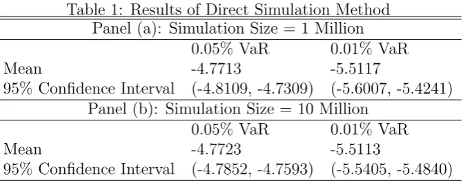
compare two different simulation sizes n = 1 million and 10 millions. Table 1 provides
the resulting mean and 95% confidence interval of the estimated 0.05% and 0.01% VaRs
across the 1,000 independent repetitions.
When the simulation size n= 1 million, a single run of the direct simulation method
is likely to produce 0.05% VaR estimate ranging from -$4.81 units to -$4.73 units based
on its 95% confidence interval, while the true 0.05% VaR is about -$4.77 units. For the
more extreme 0.01% VaR, the possible estimates in a single run of the direct simulation
method could diverge even further, from -$5.60 units to -$5.42 units based on its 95%
confidence interval. When the simulation sizen increases to 10 millions, which is a rather
4
To apply the result in Craig (1936) which is for the product of two independent normal vari-ables, we can define W = −ρσy
σx
X +Y, which is independent of X by construction, and rewrite Z = (F0+
ρσy
σx E0
)
X +E0W +X W + ρσy
σx
X2. Even though we know the CDF of X W based on
Table 1: Results of Direct Simulation Method Panel (a): Simulation Size = 1 Million
0.05% VaR 0.01% VaR
Mean -4.7713 -5.5117
95% Confidence Interval (-4.8109, -4.7309) (-5.6007, -5.4241) Panel (b): Simulation Size = 10 Million
0.05% VaR 0.01% VaR
Mean -4.7723 -5.5113
95% Confidence Interval (-4.7852, -4.7593) (-5.5405, -5.4840)
large simulation sample rarely used in practice, the 0.01% VaR estimate could still show
about $0.06 units of variation based on its 95% confidence interval.
For the proposed conditional method, we select the change of exchange rate Y as the
conditioning variable since its variance is smaller than that of the foreign currency earning
X. It follows that X|Y =y ∼ N(µx|y, σx2|y
)
, where µx|y = ρσσx
y y and σx|y =
√
1−ρ2σ
x.
Armed with the conditional distribution of X, Equation (5) can be adaptd to solve for
the VaRs. Nevertheless, in the case of a bivariate normal distribution for X and Y,
the distribution of the structural exchange rate risk Z conditional on Y = y is directly
available asN(µz|y, σz2|y
)
, whereµz|y =E0y+ (F0+y)ρσσx
y yand σz|y =|F0+y|
√
1−ρ2σ
x.
This conditional distribution of Z can be directly inserted into Equation(3) to estimate
the VaRs.
To solve Equation(6), we set the convergence criterion of the equation solver to be
that the left side of Equation(6) is within the range ofp±1e-6. The grid of the numerical
integration is selected to be from -12 to 12, which results inπ = 0.01%. That is, more than
1−π = 99.99% of the possible values of Y is covered by this grid. The grid step size is
0.01, which results 2,401 grid points in the numerical integration. The resulting estimate
of the 0.05% and 0.01% VaRs is -$4.7723 units and -$5.5118 units respectively, very
close to the corresponding average VaR estimates across 1,000 independent repetitions
by the direct simulation method. Changing the grid step size to be 0.001 or the grid
coverage probability to be π = 0.001% has little impact on the VaR estimates, resulting
4
Conclusion
Given the distributions of the foreign currency earningX and the change of exchange rate
Y, this paper proposes a conditional method to estimate VaRs of the structural exchange
rate risk that imply extremely high survival probabilities of usually more than 99.9%.
Compared with the direct simulation method that directly calculates the tail percentiles
of simulations from the joint distribution of X and Y, the conditional method produces
numerically more stable estimate of the extreme VaRs by solving a non-linear equation
via a simple one-dimensional numerical integration. The proposed conditional method is
generally applicable as long as the CDF of eitherX orY conditional on the other variable
has a closed-form expression. The bivariate normal and Student’s t distributions fall into
this category.
References
Craig, C.(1936): “On the frequency function of xy,” Annals of Mathematical Statistics,
7, 1–15.
Jackson, P., W. Perraudin, and V. Sapporta (2004): “Regulatory and economic
solvency standards for internationally active banks,” Journal of Banking and Finance,
26, 953–976.
Kotz, S.,and S. Nadarajah(2004): Multivariate t distribution and their applications.
Cambridge University Press.
KPMG (2004): “Basel II - a closer look: managing economic capital,” Discussion paper,
KPMG International.
Papaioannou, M. (2006): “Exchange risk measurement and management: issues and
approaches for firms,” Discussion paper, International Monetary Fund, Working Paper
Roth, M.(2013): “On the Multivariate t Distribution,” Discussion paper, Department of
Electrical Engineering, Linkopings Universitet, Sweden, Report No. LiTH-ISY-R-3059.
Seijas-Macias, A.,andA. Oliveira(2012): “An approach to distribution of the
prod-uct of two normal variables,” Discussiones Mathematicae - Probability and Statistics,
32, 87–99.
Wallgren, C. (1980): “The distribution of the product of two correlated t variates,”