Unsupervised Bilingual POS Tagging with Markov Random Fields

Proceedings of EMNLP 2011, Conference on Empirical Methods in Natural Language Processing, pages 64–71,

Unsupervised Bilingual POS Tagging with Markov Random Fields

Desai Chen Chris Dyer Shay B. Cohen Noah A. Smith School of Computer Science

Carnegie Mellon University Pittsburgh, PA 15213, USA

desaic@andrew.cmu.edu, {cdyer,scohen,nasmith}@cs.cmu.edu

Abstract

In this paper, we give a treatment to the prob-lem of bilingual part-of-speech induction with parallel data. We demonstrate that na¨ıve op-timization of log-likelihood with joint MRFs suffers from a severe problem of local max-ima, and suggest an alternative – using con-trastive estimation for estimation of the pa-rameters. Our experiments show that estimat-ing the parameters this way, usestimat-ing overlappestimat-ing features with joint MRFs performs better than previous work on the1984dataset.

1 Introduction

This paper considers unsupervised learning of lin-guistic structure—specifically, parts of speech—in parallel text data. This setting, and more gener-ally the multilingual learning scenario, has been found advantageous for a variety of unsupervised NLP tasks (Snyder et al., 2008; Cohen and Smith, 2010; Berg-Kirkpatrick et al., 2010; Das and Petrov, 2011).

We consider globally normalized Markov random fields (MRFs) as an alternative to directed models based on multinomial distributions or locally nor-malized log-linear distributions. This alternate pa-rameterization allows us to introduce correlated fea-tures that, at least in principle, depend on any parts of the hidden structure. Such models, sometimes called “undirected,” are widespread in supervised

NLP; the most notable instances are conditional ran-dom fields (Lafferty et al., 2001), which have en-abled rich feature engineering to incorporate knowl-edge and improve performance. We conjecture that

the “features view” of NLP problems is also more appropriate in unsupervised settings than the con-trived, acyclic causal stories required by directed models. Indeed, as we will discuss below, previous work on multilingual POS induction has had to re-sort to objectionable independence assumptions to avoid introducing cyclic dependencies in the causal network.

While undirected models are formally attractive, they are computationally demanding, particularly when they are used generatively, i.e., as joint dis-tributions over input and output spaces. Inference and learning algorithms for these models are usually intractable on realistic datasets, so we must resort to approximations. Our emphasis here is primarily on the machinery required to support overlapping fea-tures, not on weakening independence assumptions, although we weaken them slightly. Specifically, our parameterization permits us to model the relation-ship between aligned words in any configuration, rather than just those that conform to an acyclic gen-erative process, as previous work in this area has done (§2). We incorporate word prefix and suffix features (up to four characters) in an undirected ver-sion of a model designed by Snyder et al. (2008). Our experiments suggest that feature-based MRFs offer advantages over the previous approach.

2 Related Work

in which aligned words share states (a fixed and observable word alignment is assumed). Figure 1 gives an example for a French-English sentence pair. Following Goldwater and Griffiths (2007), the tran-sition, emission and coupling parameters are gov-erned by Dirichlet priors, and a token-level col-lapsed Gibbs sampler is used for inference. The hy-perparameters of the prior distributions are inferred from data in an empirical Bayesian fashion.

Why repeat that catastrophe ?

Pourquoi répéter la même catastrophe ? x1/y1 X2/y2

y3 y4

x5/y6 x4/y5

x3

Figure 1: Bilingual Directed POS induction model

When word alignments are monotonic (i.e., there are no crossing links in the alignment graph), the model of Snyder et al. is straightforward to con-struct. However, crossing alignment links pose a problem: they induce cycles in the tag sequence graph, which corresponds to an ill-defined probabil-ity model. Their solution is to eliminate such align-ment pairs (their algorithm for doing so is discussed below). Unfortunately, this is a potentially a seri-ous loss of information. Crossing alignments often correspond to systematic word order differences be-tween languages (e.g., SVO vs. SOV languages). As such, leaving them out prevents useful information about entire subsets of POS types from exploiting of bilingual context.

In the monolingual setting, Smith and Eisner (2005) showed similarly that a POS induction model can be improved with spelling features (prefixes and suffixes of words), and Haghighi and Klein (2006) describe an MRF-based monolingual POS induction model that uses features. An example of such a monolingual model is shown in Figure 2. Both pa-pers developed different approximations of the com-putationally expensive partition function. Haghighi and Klein (2006) approximated by ignoring all sen-tences of length greater than some maximum, and the “contrastive estimation” of Smith and Eisner (2005) approximates the partition function with a set

Economic discrepancies

A N

are

V

growing

V

Figure 2: Monolingual MRF tag model (Haghighi and Klein, 2006)

of automatically distorted training examples which are compactly represented in WFSTs.

Das and Petrov (2011) also consider the prob-lem of unsupervised bilingual POS induction. They make use of independent conventional HMM mono-lingual tagging models that are parameterized with feature-rich log-linear models (Berg-Kirkpatrick et al., 2010). However, training is constrained with tag dictionaries inferred using bilingual contexts derived from aligned parallel data. In this way, the complex inference and modeling challenges associated with a bilingual tagging model are avoided.

Finally, multilingual POS induction has also been considered without using parallel data. Cohen et al. (2011) present a multilingual estimation technique for part-of-speech tagging (and grammar induction), where the lack of parallel data is compensated by the use of labeled data for some languages and unla-beled data for other languages.

3 Model

Our model is a Markov random field whose ran-dom variables correspond to words in two parallel sentences and POS tags for those words. Lets =

hs1, . . . , sNsiandt = ht1, . . . , tNtidenote the two

word sequences; these correspond toNs +Nt

ob-served random variables.1 Letxandydenote the se-quences of POS tags forsandt, respectively. These are the hidden variables whose values we seek to in-fer. We assume that a word alignment is provided for the sentences. LetA ⊆ {1, . . . , Ns} × {1, . . . Nt}

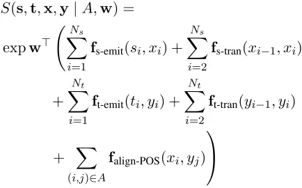
denote the word correspondences specified by the alignment. The MRF’s unnormalized probabilityS

1_{We use “source” and “target” but the two are completely}

assigns:

S(s,t,x,y|A,w) =

expw>

Ns

X

i=1

fs-emit(si, xi) + Ns

X

i=2

fs-tran(xi−1, xi)

+

Nt

X

i=1

ft-emit(ti, yi) + Nt

X

i=2

ft-tran(yi−1, yi)

+ X

(i,j)∈A

falign-POS(xi, yj)





where w is a numerical vector of feature weights that parameterizes the model. Each f• corre-sponds to features on pairs of random variables; a source POS tag and word, two adjacent source POS tags, similarly for the target side, and aligned source/target POS pairs. For simplicity, we letf de-note the sum of these five feature vectors. (In most settings, each feature/coordinate will be specific to one of the five addends.) In this paper, the features are indicators for each possible value of the pair of random variables, plus prefix and suffix features for words (up to four characters). These features encode information similar to the Bayesian bilingual HMM discussed in§2. Future work might explore exten-sions to this basic feature set.

The marginal probability of the words is given by:

p(s,t|A,w) =

P

x,yS(x,y,s,t|A,w) P

s0_,t0P_x,yS(s0,t0,x,y|A,w)

.

Maximum likelihood estimation would choose weights wto optimize a product of quantities like the above, across the training data.

A key advantage of this representation is that any alignments may be present. In directed models, crossing links create forbidden cycles in the graph-ical model. For example, Figure 3 shows a cross-ing link between “Economic discrepancies” and “di-vergences economiques.” Snyder et al. (2008) dealt with this problem by deleting word correspondences that created cycles. The authors deleted crossing links by considering each alignment link in the order of the source sentence, deleting it if it crossed pre-vious links. Deleting crossing links removes some information about word correspondence.

divergences économiques

Economic discrepancies

N A

A N Les

ART

vont

are

V

V

croissant

growing

V

V

Figure 3: Bilingual tag model.

4 Inference and Parameter Learning

When using traditional generative models, such as hidden Markov models, the unsupervised setting lends itself well to maximizing joint log-likelihood, leading to a model that performs well (Snyder et al., 2008). However, as we show in the following analysis, maximizing joint log-likelihood for a joint Markov random field with arbitrary features suffers from serious issues which are related to the com-plexity of the optimized objective surface.

4.1 MLE with Gradient Descent

For notational simplicity, we assume a single pair of sentencessandt; generalizing to multiple training instances is straightforward. The marginalized log-likelihood of the data givenwis

L(w) = logp(s,t|w)

= log

P

x,yS(x,y,s,t|w) P

s0_,t0P_x,yS(x,y,s0,t0 |w)

.

In general, maximizing marginalized log-likelihood is a non-concave optimization problem. Iterative hill-climbing methods (e.g., expectation-maximization and gradient-based optimization) will lead only to local maxima, and these may be quite shallow. Our analysis suggests that the problem is exacerbated when we move from directed to undirected models. We next describe a simple experiment that gives insight into the problem.

maximized the marginalized log-likelihood for two models: a hidden Markov model and an MRF. Both use the same set features, only the MRF is globally normalized. The number of hidden states in both models is 4.

The global maximium in both cases would be achieved when the emission probabilities (or feature weights, in the case of MRF) map each observation symbol to a single state. When we tested whether this happens in practice, we noticed that it indeed happens for hidden Markov models. The MRF, how-ever, tended to use fewer than four tags in the emis-sion feature weights, i.e., for half of the tags, all emission feature weights were close to 0. This ef-fect also appeared in our real data experiments.

The reason for this problem with the MRF, we be-lieve, is that the parameter space of the MRF is un-derconstrained. HMMs locally normalize the emis-sion probabilities, which implies that a tag cannot “disappear”—a total probability mass of 1 must al-ways be allocated to the observation symbols. With MRFs, however, there is no such constraint. Fur-ther, effective deletion of a state yrequires zeroing out transition probabilities from all other states to

y, a large number of parameters that are completely decoupled within the model.

30 35 40 45 50 55 60 65 70 75 80 85 0

20 40 60 80 100 120 140

1607 6 5 4 3

(a) likelihood

0.11 0.12 0.13 0.14 0.15 0.16 0.17 0.18 0.19 3 4 5 6 0

20 40 60 80 100 120 140 160

180 5 4-7 3-5 4-5

(b) contrastive objective

Figure 4: Histograms of local optima found by opti-mizing the length neighborhood objective (a) and the contrastive objective (b) on a synthetic dataset with 8 sentences of length 7. The weights are initialized uniformly at random in the interval[−1,1]. We plot frequency versus negated log-likelihood (lower hor-izontal values are better). An HMM always finds a solution that uses all available tags. The numbers at the top are numbers of tags used by each local opti-mum.

Our bilingual model is more complex than the

above example, and we found in preliminary exper-iments that the effect persists there, as well. In the following section, we propose a remedy to this prob-lem based on contrastive estimation (Smith and Eis-ner, 2005).

4.2 Contrastive Estimation

Contrastive estimation maximizes a modified ver-sion of the log-likelihood. In the modified verver-sion, it is the normalization constant of the log-likelihood that changes: it is limited to a sum over possible ele-ments in aneighborhoodof the observed instances. More specifically, in our bilingual tagging model, we would define a neighborhood function for sen-tences, N(s,t) which maps a pair of sentences to a set of pairs of sentences. Using this neighborhood function, we maximize the following objective func-tion:

Lce(w)

= logp(S=s,T=t|S∈N1(s),T∈N2(t),w)

= log

P

x,yS(s,t,x,y|w) X

s0_,t0_∈N(s,t) X

x,y

S(s0,t0,x,y|w).

(1) We define the neighborhood function using a cross-product of monolingual neighborhoods:

N(s,t) = N1(s)×N1(t). N1is the “dynasearch” neighborhood function (Potts and van de Velde, 1995; Congram et al., 2002), used for contrastive estimation previously by Smith (2006). This neigh-borhood defines a subset of permutations of a se-quences, based on local transpositions. Specifically, a permutation of s is in N1(s) if it can be derived fromsthrough swaps of any adjacent pairs of words, with the constraint that each word only be moved once. This neighborhood can be compactly repre-sented with a finite-state machine of sizeO(Ns)but

encodes a number of sequences equal to the Nsth

Fibonacci number.

Monolingual Analysis To show that contrastive

we compare the maxima identified using MLE with the monolingual MRF model to the maxima identi-fied by contrastive estimation. The results are con-clusive: MLE tends to get stuck much more often in local maxima than contrastive estimation.

Following an analysis of the feature weights found by contrastive estimation, we found that con-trastive estimation puts more weight on the transi-tion features than emission features, i.e., the tran-sition features weights have larger absolute values than emission feature weights. We believe that this could explain why contrastive estimation finds better local maximum that plain MLE, but we leave explo-ration of this effect for future work.

It is interesting to note that even though the con-trastive objective tends to use more tags available in the dictionary than the likelihood objective does, the maximum objective that we were able to find does not correspond to the tagging that uses all available tags, unlike with HMM, where the maximum that achieved highest likelihood also uses all available tags.

4.3 Optimizing the Contrastive Objective

To optimize the objective in Eq. 1 we use a generic optimization technique based on the gradient. Using the chain rule for derivatives, we can derive the par-tial derivative of the log-likelihood with respect to a weightwi:

∂Lce(w)

∂wi

=Ep(X,Y|s,t,w)[fi]

− _{Ep(S,T,X,Y|S∈N1(s),T∈N1(t),w)}[fi]

The second term corresponds to a computationally expensive inference problem, because of the loops in the graphical model. This situation is differ-ent from previous work on linear chain-structured MRFs (Smith and Eisner, 2005; Haghighi and Klein, 2006), where exact inference is possible. To over-come this problem, we use Gibbs sampling to obtain the two expectations needed by the gradient. This technique is closely related to methods like stochas-tic expectation-maximization (Andrieu et al., 2003) and to contrastive divergence (Hinton, 2000).

The training algorithm iterates between sam-pling part-of-speech tags and samsam-pling permutations of words to compute the expected value of fea-tures. To sample permutations, the sampler iterates

through the sentences and decides, for each sen-tence, whether to swap a pair of adjacent tags and words or not. The Markov blanket for computing the probability of swapping a pair of tags and words is shown in Figure 5. We run the algorithm for a fixed number (50) of iterations. By testing on a de-velopment set, we observed that the accuracy may increase after50iterations, but we chose this small number of iterations for speed.

N A

divergences économiques

A N

Economic discrepancies

V vont

N A

divergences économiques

A N

Economic discrepancies

ART Les

V vont

are V

Figure 5: Markov blanket of a tag (left) and of a pair of adjacent tags and words (right).

In preliminary experiments we considered stochastic gradient descent, with online updating. We found this led to low-accuracy local optima, and opted for gradient descent with batch updates in our implementation. The step size was chosen to limit the maximum absolute value of the update in any weight to0.1. Preliminary experiments showed only harmful effects from regularization, so we did not use it. These issues deserve further analysis and experimentation in future research.

5 Experiments

We next describe experiments using our undirected model to unsupervisedly learn POS tags.

With unsupervised part-of-speech tagging, it is common practice to use a full or partial dictionary that maps words to possible part-of-speech tags. The goal of the learner is then to discern which tag a word should take among the tags available for that word. Indeed, in all of our experiments we make use of a tag dictionary. We consider both a com-pletetag dictionary, where all of the POS tags for all words in the data are known,2and a smaller tag dic-tionary that only provides possible tags for the 100

2_{Of course, additional POS tags may be possible for a given}

most frequent words in each language, leaving the other words completely ambiguous. The former dic-tionary makes the problem easier by reducing ambi-guity; it also speeds up inference.

Our experiments focus on the Orwell novel1984

dataset for our experiments, the same data used by Snyder et al. (2008). It consists of parallel text of the 1984novel in English, Bulgarian, Slovene and Serbian (Erjavec, 2004), totalling 5,969 sentences in each language. The1984datset uses fourteen part-of-speech tags, two of which denote punctuation. The tag sets for English and other languages have minor differences in determiners and particles.

We use the last 25% of sentences in the dataset as a test set, following previous work. The dataset is manually annotated with part-of-speech tags. We use automatically induced word alignments using Giza++ (Och and Ney, 2003). The data show very regular patterns of tags that are aligned together: words with the same tag in two languages tend to be aligned with each other.

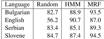
When a complete tag dictionary derived from the Slavic language data is available, the level of ambi-guity is very low. The baseline of choosing random tags for each word gives an accuracy in the low 80s. For English, we use an extended tag dictionary built from the Wall Street Journal and the1984data. The English tag dictionary is much more ambiguous be-cause it is obtained from a much larger dataset. The random baseline gives an accuracy of around 56%. (See Table 1.)

In our first set of experiments (§5.1), we perform a “sanity check” with a monolingual version of the MRF that we described in earlier sections. We com-pare it against plain HMM to assure that the MRFs behave well in the unsupervised setting.

In our second set of experiments (§5.2), we com-pare the bilingual HMM model from Snyder et al. (2008) to the joint MRF model. We show that using an MRF has an advantage over an HMM model in the partial tag dictionary setting.

5.1 Monolingual Experiments

We turn now to two monolingual experiments that verify our model’s suitability for the tagging prob-lem.

Language Random HMM MRF

Bulgarian 82.7 88.9 93.5

English 56.2 90.7 87.0

Serbian 83.4 85.1 89.3

Slovene 84.7 87.4 94.5

Table 1: Unsupervised monolingual tagging accura-cies with complete tag dictionary on1984data.

Supervised Learning As a very primitive

com-parison, we trained a monolingual supervised MRF model to compare to the results of supervised HMMs. The training procedure is based on sam-pling, just like the unsupervised estimation method described in§4.3. The only difference is that there is no need to sample the words because the tags are the only random variables to be marginalized over. Our model and HMM give very close performance with difference in accuracy less than 0.1%. This shows that the MRF is capable of representing an equiva-lent model represented by the HMM. It also shows that gradient descent with MCMC approximate in-ference is capable of finding a good model with the weights initialized to all0s.

Unsupervised Learning We trained our model

under the monolingual setting as a sanity check for our approximate training algorithm. Our model un-der monolingual mode is exactly the same as the models introduced in§2. We ran our model on the

1984data with the complete tag dictionary. A com-parison between our result and monolingual directed model is shown in Table 1. “Random” is obtained by choosing a random tag for each word according to the tag dictionary. “HMM” is a Bayesian HMM im-plemented by (Snyder et al., 2008). We also imple-mented a basic (non-Bayesian) HMM. We trained the HMM with EM and obtained rsults similar to the Bayesian HMM (not shown).

5.2 Billingual Results

Re-Language pair HMM MRF MRF w/o cross. MRF w/o spell.

English 71.3 73.3±0.6 73.4±0.6 67.4±0.9

Bulgarian 62.6 62.3±0.3 63.8±0.4 55.2±0.5

Serbian 54.1 55.7±0.2 54.6±0.3 47.7±0.5

Slovene 59.7 61.4±0.3 60.4±0.3 56.7±0.4

English 66.5 73.3±0.3 73.4±0.2 62.3±0.5

Slovene 53.8 59.7±2.5 57.6±2.0 52.1±1.3

Bulgarian 54.2 58.1±0.1 56.3±1.3 58.0±0.2

Serbian 56.9 58.6±0.3 59.0±1.2 55.1±0.3

English 68.2 72.8±0.6 72.7±0.6 65.7±0.4

Serbian 54.7 58.5±0.6 57.7±0.3 54.2±0.3

Bulgarian 55.9 59.8±0.1 60.3±0.5 55.0±0.4

Slovene 58.5 61.4±0.3 61.6±0.4 58.1±0.6

Average 59.7 62.9 62.5 56.5

Table 2: Unsupervised bilingual tagging accuracies with tag dictionary only for the top 100 frequent words. “HMM” is the result reported by (Snyder et al., 2008). “MRF” is our contrastive model averaged over ten runs. “MRF w/o cross.” is our model trained without crossing links, like Snyder et al.’s HMM. “MRF w/o spell.” is our model without prefix and suffix features. Numbers appearing next to results are standard deviations over the ten runs.

Language w/ cross. w/o cross.

French 73.8 70.3

English 56.0 59.2

Table 3: Effect of removing crossing links when learning French and English in a bilingual setting.

moving the prefix and suffix features gives substan-tially lower results on average, results even below plain HMMs.

The reason that crossing links do not change the results much could be related to fact that most of the sentence pairs in the1984dataset do not contain many crossing links (only 5% of links cross another link). To see whether crossing links do have an ef-fect when they come in larger number, we tested our model on French-English data. We aligned 10,000 sentences from the Europarl corpus (Koehn, 2005), resulting in 87K crossing links out of a total of 673K links. Using the Penn treebank (Marcus et al., 1993) and the French treebank (Abeill´e et al., 2003) to evaluate the model, results are given in Table 3. It is evident that crossing links have a larger effect here, but it is mixed: crossing links improve performance for French while harming it for English.

6 Conclusion

In this paper, we explored the capabilities of joint MRFs for modeling bilingual part-of-speech mod-els. Exact inference with dynamic programming is not applicable, forcing us to experiment with ap-proximate inference techniques. We demonstrated that using contrastive estimation together with Gibbs sampling for the calculation of the gradient of the objective function leads to better results in unsuper-vised bilingual POS induction.

Our experiments also show that the advantage of using MRFs does not necessarily come from the fact that we can use non-monotonic alignments in our model, but instead from the ability to use overlap-ping features such as prefix and suffix features for the vocabulary in the data.

Acknowledgments

References

A. Abeill´e, L. Cl´ement, and F. Toussenel. 2003. Building a treebank for French. In A. Abeill´e, editor,Treebanks. Kluwer, Dordrecht.

C. Andrieu, N. de Freitas, A. Doucet, and M. I. Jordan. 2003. An introduction to MCMC for machine

learn-ing. Machine Learning, 50:5–43.

T. Berg-Kirkpatrick, A. Bouchard-Cote, J. DeNero, and D. Klein. 2010. Unsupervised learning with features.

InProceedings of NAACL.

S. B. Cohen and N. A. Smith. 2010. Covariance in unsu-pervised learning of probabilistic grammars. Journal

of Machine Learning Research, 11:3017–3051.

S. B. Cohen, D. Das, and N. A. Smith. 2011. Unsuper-vised structure prediction with non-parallel multilin-gual guidance. InProceedings of EMNLP.

R. K. Congram, C. N. Potts, and S. L. van de Velde. 2002. An iterated Dynasearch algorithm for the single-machine total weighted tardiness scheduling problem. Informs Journal On Computing, 14(1):52– 67.

D. Das and S. Petrov. 2011. Unsupervised part-of-speech tagging with bilingual graph-based projections.

InProcedings of ACL.

T. Erjavec. 2004. MULTEXT-East version 3: Multilin-gual morphosyntactic specifications, lexicons and cor-pora. InProceedings of LREC.

S. Goldwater and T. Griffiths. 2007. A fully Bayesian approach to unsupervised part-of-speech tagging. In

Proc. of ACL.

A. Haghighi and D. Klein. 2006. Prototype-driven learn-ing for sequence models. In Proceedings of

HLT-NAACL.

G. E. Hinton. 2000. Training products of experts by minimizing contrastive divergence. Technical Report GCNU TR 2000-004, University College London. P. Koehn. 2005. Europarl: A parallel corpus for

statisti-cal machine translation. InMT Summit 2005.

J. D. Lafferty, A. McCallum, and F. C. N. Pereira. 2001. Conditional random fields: Probabilistic models for segmenting and labeling sequence data. In

Proceed-ings of ICML.

M. P. Marcus, B. Santorini, and M. A. Marcinkiewicz. 1993. Building a large annotated corpus of En-glish: The Penn treebank. Computational Linguistics, 19:313–330.

F. Och and H. Ney. 2003. A systematic comparison of various statistical alignment models. Computational

Linguistics, 29(1):19–51.

C. N. Potts and S. L. van de Velde. 1995. Dynasearch– iterative local improvement by dynamic programming. Part I: The traveling salesman problem. Technical re-port.

N. A. Smith and J. Eisner. 2005. Contrastive estimation: training log-linear models on unlabeled data. InProc. of ACL.

N. A. Smith. 2006.Novel Estimation Methods for Unsu-pervised Discovery of Latent Structure in Natural

Lan-guage Text. Ph.D. thesis, Johns Hopkins University.