Munich Personal RePEc Archive
Non-Radial Directional Performance
Measurement with Undesirable Outputs
Chen, Po-Chi and Yu, Ming-Miin and Chang, Ching-Cheng
and Managi, Shunsuke
Department of International Business, Chung Hua University,
Hsinchu, Taiwan, Department of Transportation Science, National
Taiwan Ocean University, Keelung, Taiwan, Institute of Economics,
Academia Sinica, Taipei, Taiwan, Graduate School of Environmental
Studies, Tohoku University, Sendai, Japan
2014
Online at
https://mpra.ub.uni-muenchen.de/57189/
Non-Radial Directional Performance Measurement with Undesirable Outputs
Po-Chi Chena, Ming-Miin Yub,*, Ching-Cheng Changc, and Shunsuke Managid*
aDepartment of International Business, Chung Hua University, Hsinchu, Taiwan
bDepartment of Transportation Science, National Taiwan Ocean University, Keelung, Taiwan cInstitute of Economics, Academia Sinica, Taipei, Taiwan
dGraduate School of Environmental Studies, Tohoku University, Sendai, Japan (* corresponding author)
Abstract
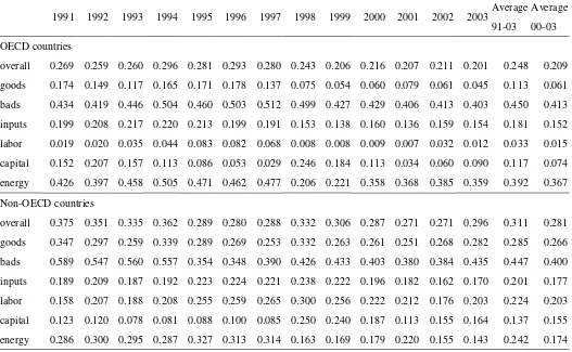
The objective of this paper is to provide a comprehensive efficiency measures to estimate the performances of OECD and non-OECD countries. A Russell directional distance function that appropriately credits the decision making unit not only for increase in desirable outputs but also for the decrease of undesirable outputs is derived from the proposed weighted Russell directional distance model. The method was applied to a panel of 99 countries over 1991 and 2003. This framework also decomposes the comprehensive efficiency measure into individual input/output components’ inefficiency scores that are useful for policy making. The results reveal that the OECD countries perform better than the non-OECD countries in overall, goods, labor and capital efficiencies, but worse in bad and energy efficiencies.
1. Introduction
It has long been recognized in the technical efficiency literature that data envelopment analysis (DEA) is particularly adept at computing multiple input and output production correspondences (Seiford and Zhu, 1999). Generally, there are two types of measure in DEA, namely radial and non-radial (Tone, 2010). Radial measures are represented by CCR (Charnes et al., 1978) and BCC (Banker et al., 1984) models. However, because radial measures of efficiency overestimate technical efficiency when there are non-zero slacks in the constraints defining the piece-wise linear technology (Fukuyama and Weber, 2009), recent research has sought to construct alternative non-radial efficiency measures that account for slacks.
In the literature of the non-radial models, the proposed methods can be roughly divided into the following three groups: (1) the Russell measure, which was first presented by Färe and Lovell (1978) with an input-oriented form. Nevertheless, it only accounts for all the slacks of inputs, but fails to consider the inefficiencies associated with outputs. It was later extended by Färe et al. (1985) in a nonlinear form that they refer to as the “Russell graph measure”, which combines the input and output Russell measures in an additive way and accounts for all the input slacks as well as the output slacks. Pastor et al. (1999) then further revised it to a new measure called the “Enhanced Russell graph measure” (ERGM), which in turn combines input and output Russell measures in a ratio form. (2) the additive model, which was developed by Charnes et al. (1985) and also accounts for all sources of inefficiency both in inputs and outputs. However, it does not directly provide an efficiency measure (Pastor et al., 1999). (3) the slacks-based model (SBM), which was proposed by Tone (2001) with the objective of maximizing all the input and output slacks in fractional programming form. Cooper et al. (2007) showed that SBM is equivalent to ERGM.
Recently, Fukuyama and Weber (2009) introduced the directional distance function technology into SBM to develop a generalized measure of technical inefficiency which also accounts for all slacks in input and output constraints. This new measure was referred to as the directional slacks-based inefficiency (SBI) measure. This is shown to yield the same information on performance as Tone’s SBM of efficiency when the directional vectors for inputs and outputs are chosen to equal the actual input and output vector, and can also be thought of as a generalization of the original Russell measure of efficiency. On the other hand, Färe and Grosskopf (2010) also proposed a generalization of the SBM measure based on the directional distance function. The optimization problem of this measure is based on the sum of directional distance function and can tell how much excess inputs have been employed and how much outputs short of an efficient level have been produced.
jointly1. It is therefore reasonable to consider not only all the inefficiency sources of inputs and desirable outputs but also all the inefficiency sources of undesirable outputs when we evaluate the performance of a decision making unit (DMU). To our knowledge, both Zhou et al. (2006) and Zhou et al. (2007) had extended the SBM and Russell measure to incorporate undesirable outputs. Nevertheless, the models established in the former one do not really account for all the inefficiency sources of undesirable outputs. The models constructed in the latter study only measure the performance of undesirable outputs (referred to as a Russell environmental performance index in Zhou et al., 2007) and thus ignore the inefficiency sources of inputs and desirable outputs.
The purpose of this study is to extend the directional Russell measure of inefficiency proposed by Fukuyama and Weber (2009) into the cases where undesirable outputs exist. We refer to the proposed model as the weighted Russell directional distance model (WRDDM).2 Compared to the
original SBM and ERGM, which combine input and output efficiency measures in a nonlinear fractional form, our directional distance function based measure is evaluated in linear form and hence possesses the attractive advantages of easy computation and easy extension of incorporating the additional undesirable outputs into the programming problems.
The remainder of this paper is organized as follows. The next section presents the model. For comparison purpose, we first illustrate the traditional directional distance function model (TDDFM) problem, which credits a producer for simultaneously increasing production of the good output, reducing production of bad outputs and contracting employment of inputs. Then, the extended models are followed. The SBM and Russell measure, which correspond to our WRDDM, are also presented. Section three demonstrates using a case study of panel data of 99 countries. Our measure obtained is easily decomposed into separate measures of input, desirable and undesirable output efficiencies, and can help us to shed more light on the sources of inefficiencies. In the case of the environmental issues are evaluated, it provides us an integrated measure of economic and environmental performance. The final section concludes.
2. Preliminary
2.1 The Traditional Directional Distance Function Model
Let inputs be denoted by x∈RN, good outputs by yRM , and bad or undesirable outputs by bRJ, where R represents the non-negative Euclidean *-orthant. The directional distance function seeking to increase the desirable outputs and decrease the undesirable outputs and inputs directionally can be defined by the following formulation:
1 As Smith (1990) pointed out, undesirable outputs may also appear in health care (e.g. complications of medical operations) and business (e.g. tax payments) applications.
) ; , ,
(x y b g
D =sup{: (xgx, yg by, gb)T}, (1)
where the non-zero vector g(gx,gy,gb) determines the “directions” in which inputs, desirable outputs and undesirable outputs are scaled, and the technology reference set
)} , ( : ) , ,
{(x y b xcan produce y b
T satisfies the assumptions of constant returns to scale, strong disposability of inputs, and weak disposability of both desirable outputs and undesirable outputs.
Suppose there are k 1,,K DMUs in the data set. Each DMU uses input N k N k k k R x x x
x ( 1, 2,, ) to jointly produce desirable outputs
M k M k k k R y y y
y ( 1, 2,, ) and
undesirable outputs k J
J k k k R b b b
b ( 1 , 2,, ) . The DEA piecewise reference technology can be constructed as follows:
T={( x, y, b): ,
1
m K
k
mk
ky y
z
m1,...,M,
,
1 j
K k k jk
b b
z
j1,...,J,
,
1 n
K k k nk
x x
z
n1, . . . .N, (2)
, 0
k
z k 1, . . . .K},
where zk are the intensity variables to shrink or expand the individual observed activities of DMU k for the purpose of constructing convex combinations of the observed inputs and outputs.
Relative to the reference technology T constructed in (2), traditionally, for each DMU K
k1,, , the directional distance function can be obtained by solving the following linear programming problem3:
( k, k , k; ) max k D x y b g
s.t. ' '
1
,
m
K
k
k mk mk y
k
z y y g
m1, . . . .M,'
' ,
1 j
K
k
k jk jk b
k
z b b g
j1, . . . .J,' ' 1 , n K k
k nk nk x
k
z x x g
n1, . . . .N, (3), 0
k
z k 1, . . . .K
3 A referee reminds that it is still debating about variable return to scale in weakly disposable technology. Thus, the efficiency is evaluated with variable returns to scale technology, it needs not only to impose the additional constraint
of 1
1
K k kwhere k
measures the maximum expansion of desirable outputs and contraction of undesirable
outputs and inputs that remain technically feasible and can serve as a measure of technical
inefficiency. If k 0
, then DMU k operates on the frontier of T with technical efficiency. If k 0
, then DMU k operates inside the frontier of T.
Other than being the generalization of the Shephard’s distance functions4, one of the important
characteristics of the directional distance function is that the direction in which performance is scaled can be specified flexibly to accommodate different analysis purposes. For example, if we set
) , ,
( gx gy gb
g =(xk',yk',bk'), i.e., the direction is chosen based on the observed data, k represents the potential proportionate change in goods, bads and inputs. If instead we take
) , ,
( gx gy gb
g =(1,1,1), then we can interpret the solution value as the net improvement in performance in terms of feasible increase in goods outputs and feasible decreases in bad outputs and inputs (Färe and Grosskopf, 2004). On the other hand, setting g(0,gy,gb), we get the directional output (including goods and bads) distance function or environmental directional output distance function as referred to by Färe et al. (2007) (cf. Färe et al. (2007) for more details).
However, as mentioned previously, the measure of this approach fails to consider the inefficiencies associated with non-zero slacks and would have the problem of incorrectly regarding some evaluated DMUs as efficient units.
2.2. The Weighted Directional Distance Model
The efficiency measurement constructed in (3) expands all desirable outputs and contracts all inputs and undesirable outputs by the same rate of . However, there is no guarantee that the
proportional contraction (expansion) rate of for input items ( ), desirable output items ( ) and undesirable output items ( ) must be the same ( ) in practice. We believe this is a strong assumption of the model. Thus, the formulation of (3) can be generalized to accommodate different expansion and contraction scales as follows:
( , , ; ) max
w k k k k k k k
y b x w
D x y b g
s.t. '
1
,
m
K
k
k mk mk y
k
z y y g
m1, . . . .M,' ,
1 j
K
k
k jk jk b
k
z b b g
j1, . . . .J,
'
1
,
n
K
k
k nk nk x
k
z x x g
n1, . . . .N, (4), 0
k
z k 1, . . . .K
It is required that the directional vectors have same units of measurement as the vectors of the observed data, so that it allows the , , to be added. 5 The measure
( , , ; , , )
n m j
w k k k
x y b
D x y b g g g given in (4) is maximized hyperbolically
k k k k
w y b x
by comparing the observed (xnk,ymk,bkj )
with the frontier
( ( )
n
k
nk x
x g , ( )
m
k
mk y
y g , ( )
j
k
jk b
b g ). The weighted directional distance function gives the expansion in good outputs and contraction in bad outputs and inputs simultaneously. When
( , , ; , , ) 0
n m j
w k k k
x y b
D x y b g g g , DMU k’ is technically efficient because no additional improvements in good outputs, bad outputs and inputs are feasible.
( , , ; , , ) 0
n m j
w k k k
x y b
D x y b g g g indicates technical inefficiency. The coefficientsy, b and
x
are associated with the priorities or managerial preferences given to the outputs (goods and bads) and inputs and their sum is normalized to unity. The improvements for desirable outputs,
undesirable outputs, and inputs can be measured by k , k
, and k
, respectively, and then used
to calculate the weighted inefficiency score k w
.
Note that if we set kkk
, then model (4) degenerates to model (3) 6.In addition, in
the one input, one desirable output and one undesirable output case, formulation (4) is able to account for all the slacks. However, in the multiple inputs, desirable outputs and undesirable outputs case, it may still fail to identify all the non-zero slacks associated with the input and output constraints.
3. The Model
3.1. The Weighted Russell Directional Distance Model
Inspired by the equivalence of the ERGM and SBM, we follow an idea similar to that of the ERGM to generalize the traditional directional distance function and develop another similar measure called the weighted Russell directional distance model (WRDDM). It is important to note that the WRDDM is a closely related measure of ERGM, while the ERGM and SBM are special
5 This requirement is the same as what Fukuyama and Weber (2009, p276) point out, that the directional vectors have the same units of measurement as the vectors of the input and output slack, and when g =1, the role of the directional vectors is also similar to that of the el in Färe and Grosskopf (2010).
6 One of the anonymous referees reminds that considering
y
in the objective function together with
m
y g
among the constraints. The following can be done, assuming that y is strictly positive (
m m
y gy y gy
where y ,
m m
y y y
cases of the WRDDM measure7. The proposed programming model is: ) ( ) ( ) ( max ) ; , , ( 1 1 1 '
N
n k n x n x J j k j b j b M m k m y m y k R k k k R w w w g b y x
D
s.t. ' '
1 , m m K k
k mk mk y
k
z y y g
m1, . . . .M,'
' ,
1 j
K
k k jk jk j b k
z b b g
j1, . . . .J,' ' 1 , n K k k nk nk n x k
z x x g
n1, . . . .N, (5), 0
k
z k 1, . . . .K where k', k', k'
m j n
are the individual inefficiency measure for each desirable output ym, each undesirable output bj and each input xn. In other words, this specification allows for not only the technical inefficiency associated with desirable output, undesirable output and input to be different, but also allows the technical inefficiency among each of the desirable outputs, the
undesirable outputs and the inputs to be different
( k ( 1, , ) k( 1, , ) k( 1, , )
m m M j j J n n N
). This makes sense, because , for
example, the inefficiency of the input uses of a firm could be more from the inefficient use of labor (use too many workers or there is labor congestion) but less from capital. On the other hand, a producer may produce several products at the same time (e.g. crops and livestock production of farmers or loans and securities investment production of banks), but with different production ability, and hence the production efficiency for different product would be different. Therefore, one of the advantages of this model is that it can help us to identify the source where we need to improve most.
Once again,the directional vectors are required to have the same units of measurement as the
vectors of the observed data, so that it allows the k', k', k'
m j n
to be added. If the coefficients wy,
b
w and wx denote the given priorities associated with the outputs (goods and bads) and inputs, and their sum is normalized to unity, and the inefficiencies of each corresponding input (output) is also specified to allow assigning different priorities to each of it and their sums are assumed to be
one: 1 1 M y m m
, 1 1 J b j j
and1 1 N x n n
, then this is similar to what Liu and Tone (2008) did.8
7 The difference between the ERGM and the WRDDM exists in their objective functions and constraints. The objective function of the ERGM is specified for calculating efficiency measure, while those respective variables in the WRDDM are inefficiency measures. In addition, WRDDM has additive form objective function, while ERGM is ratio form and ERGM does not consider undesirable outputs (cf. Pastor et al. (1999) for more details).
8 That is, if we alternatively specify the objective function in (5) as
1 1 1
1
( )
3
M J N
y k b k x k
m m j j n n
m j n
,However, it is noted that if the direction vectors do not have the same units of measurement as the
vectors of the observed data, we can alternatively set the weights y m
, b
j
and x n
as values which can normalized the direction vectors, such as the sample standard deviations of the inputs and outputs. We will say more about this below when we discuss the unit invariant property of WRDDM.
By means of the following change of variables9, the Russell directional type inefficiency measures can be changed to the slacks-based ones.
' ' m m k k m y s g , j b k j k j g s ' ' , ' ' n n k k n x s g
wheresmk ',sjk',snk' are the desirable and undesirable outputs, and inputs slacks respectively which
cause the inefficiency for the evaluated unit k'. Then, the model can be re-expressed as follows:
) ( ) ( ) ( max ) ; , , ( 1 1 1 '
N
n x k n x n x J j b k j b j b M m y k m y m y k R k k k R n j m g s w g s w g s w g b y x
D
s.t. ' ',
1
mk mkK
k
mk
ky y s
z m1,...,M,
, 1 ' '
jk jkK
k
jk
kb b s
z j1,...,J,
, 1 ' '
nk nkK
k
nk
kx x s
z n1, . . . .N, (6)
0 , , ' ' ' nk jk mk s s
s m, j,n
, 0
k
z k 1,...,K
Because the slacks for each variable are allowed to be different, the objective in (6) can help us to reflect all inefficiencies by calculating the maximum expansion of all desirable outputs and contraction of all undesirable outputs and inputs that the model can identify. Thus, R
k
provides us
an aggregate or overall inefficiency measure of performance in a non-radial manner in which the
component of '
1 1 m
y
M M
m m k
y k k
m m
m m y
s g
in the objective of (5) or (6) corresponds to the averagedesirable output mix inefficiencies and similarly, the '
1 1 j
b
J J
j j k
b k k
j j
j j b
s g
andcase of our corresponding weighted SBM which will be introduced in section 3.2.
9 In ERGM, if considering bads, k' m k'
m k m s y , '
' j k
' '
1 1 n
x
N N
n n k
x k k
n n
n n x
s g
correspond to the average undesirable output and input mixinefficiencies respectively.
Let an optimal solution of model (6) be zk, sm k
, sj k
and snk
, the WRDDM overall
inefficiency is the weighted average of the desirable output inefficiency, k , undesirable output inefficiency, k, and input inefficiency, k. We define the WRDDM overall inefficiency measure R
k
by
k k k k
R wy wb wx
(k1, ,K ), (7)
where
1 m
y M
m m k k
m y
s g
,1 j
b J
j j k k
j b
s g
,1 n
x N
n n k k
n x
s g
.The optimal solution to this linear program (6) is an inefficiency score which measures the largest rectilinear distance from the observation being evaluated to the efficient production frontier. Therefore, we have the following definitions:
Definition 1. WRDDM desirable output efficient. If all optimal solutions of (6) satisfy k0, DMU
k’ is called desirable output efficient. This implies that the optimal slacks for the desirable outputs in (6) are all zero, i.e. smk 0( m)
.
Definition 2. WRDDM undesirable output efficient. If all optimal solutions of (6) satisfy k0, DMU
k’ is called undesirable output efficient. This implies that the optimal slacks for the undesirable outputs in (6) are all zero, i.e. sj k 0( j).
Definition 3. WRDDM input efficient.
If all optimal solutions of (6) satisfy k0, DMU
k’ is called input efficient. This implies that the optimal slacks for the inputs in (6) are all zero, i.e. snk 0( n)
.
Definition 4. WRDDM overall efficient.
undesirable outputs and inputs in (6) are all zero, i.e. smk sj ksnk 0( m j n, , ).
If the WRDDM inefficiency measure is zero, then the DMU is fully efficient. The inefficiency measure of WRDDM has the following properties:
Theorem 1. DMU k’ is WRDDM overall efficient, if and only if it is WRDDM efficient for all the desirable output efficient, undesirable output efficient and input efficient.
Proof. From the equality (7), this theorem holds.□
Theorem 2. The projected DMU o is WRDDM overall efficient. Proof.
Let an optimal solution of model (6) be zo, smo , sj o and sno . We define the projection of DMU
o as follows:
1 k
K
mo mk mo mo
k
y z y y s
(m1,...,M ),1 k
K
jo jk jo j o
k
b z b b s
( j1,...,J),1 k
K
no nk no no
k
x z x x s
(n1,...,N )Then, re-estimate the overall-efficiency of the projected DMU. Let an optimal solution of the
projected DMU be zo, smo, sj o and sno . We have:
1 k
K
mo mk mo
k
y z y s
(m1,...,M ),1 k
K
jo jk j o
k
b z b s
( j1,...,J),1 k
K
no nk no
k
x z x s
(n1,...,N )Replacing ymo ymosmo ( m1,...,M ), bjo bjo sj o
( j1,...,J ), and
no no no
x x s(n1,...,N) , we have:
1 k
K
mo mk mo mo
k
y z y s s
(m1,...,M ),1 k
K
jo jk j o j o
k
b z b s s
1
k
K
no nk no no
k
x z x s s
(n1,...,N )Corresponding to this expression we have the overall-inefficiency,
k o o o
R wy wb wx
( 1, ,
k K ), Where
1
( )
m
y M
m mo mo o
m y
s s g
1
( )
j
b J
j j o j o o
j b
s s g
1
( )
n
x N
n n o n o o
n x
s s g
If any element of
sno , sj o , sy o is positive, then it holds that o oR R
. This contradicts the
optimality of o R
. Thus, we have
0, 0, 0( , , )
no j o mo
s s s n j m . Hence, the projected DMU is overall-efficient. □
In addition, we can verify that WRDDM has the following properties:
Theorem 3. If, for any two DMUs k’ and k”, their inefficiencies simultaneously satisfy all of the three inequalities kk, kk, kkand then it holds that R R
k k
. Proof. From the equality (7), this theorem holds. □
Theorem 4. The WRDDM is translation invariant if and only if the convexity constraints imposed on the production possibility set.
Proof.
Let us translate the data set k ( ,1k 2k, , k) N
x x x x , k ( 1k, 2k, , k ) M
y y y y , k ( ,1k 2k, , k) J b b b b by introducing arbitrary constants n(n1, ,N), m(m1, ,M), j(j1, , )J to obtain new data
,( 1, , : 1, , )
k k
n n n
x x n N k K
,( 1, , : 1, , )
k k
m m m
y y m M k K
,( 1, , : 1, , )
k k
j j j
b b j J k K
Due to
1
1, K
k k
z
1
( 1, , ), K
k n n k
z n N
1
( 1, , ),
K
k m m
k
z m M
and1
( 1, , ), K
k j j
k
z j J
We observe that the first set of constraints in model (6) become
' '
1 1
( ) ,
K K
k mk m mk k mk mk m mk m
k k
z y s z y s y
m1, . . . .M,So that
'
1
, K
k mk mk mk k
z y s y
The same relationships are applicable to the second and third sets of constraints. Thus, the original
problem is translation invariant. The proof relies on the convexity constraint
1 1 K k k z
.□Definition 5. If the directional vector g(gx,gy,gb)is set to be g ( x y, ,b), then the WRDDM is called the observation directional WRDDM. □
Theorem 5. The observation directional WRDDM is units invariant. Proof.
Consider rescale desirable outputym, undesirable output bj and input xn by multiplying by the scalar m, j and n, respectively. Then the corresponding slacks of each output and input will also be rescaled by the same scalar. The objective function in model (6) will be as follows:
' ' '
' ' '
' ' '
1 1 1
1 1 1
1 1 1
( ) ( ) ( )
( ) ( ) ( )
( ) ( ) ( )
m
m j n
m
y b x
M J N
j n
m k j k n k
y b x
m m j j n n
y b x
M J N
m m k m j k n n k
y b x
m m m j m j n n n
y b x
M J N
j n
m k j k n k
y b x
m m j j n n
s s s
w w w
y b x
s s s
w w w
y b x
s s s
w w w
y b x
In addition, the translated restrictions are also equivalent to the original restrictions. The value of the objective is thus not affected, there, the observation directional WRDDM is units invariant.
□
Corollary 1. The observation directional WRDDM is units invariant and translation invariant if and only if the convexity constraints imposed on the problem.
Proof. From Theorems 4 and 5, this Corollary holds. □
WRDDM is called the unit directional WRDDM.
It is noted in this case, the k', k', k'
m j n
in the objective function in model (5) are equivalent
tosm k, sj k and snk without units, respectively, and R
k
is the weighted average of those
weighted sum of respective slacks. When all the individual weights, y, b, x
m j i
, are set to be one,
then model (5) degenerates to Färe and Grosskopf’s (2010) model (5).
Theorem 6. The unit directional WRDDM is units invariant. Proof.
The proof is similar to that of the proof of Theorem 4. □
Corollary 2. The unit directional WRDDM is units invariant and translation invariant if and only if the convexity constraints imposed on the problem.
Proof. From Theorems 4 and 6, this Corollary holds. □
Definition 7. If the directional vectors do not have the same units of measurement as the vectors of the observed data and the weights corresponding to each of the inputs, desirable and undesirable outputs are the reciprocal of sample standard deviations, the WRDDM is called the inverse variance WRDDM.10
Theorem 7. The inverse variance WRDDM is units invariant. Proof.
Let the sample standard deviations of the desirable output ym, undesirable outputbj and
input xn be y m
, b
j
and x n
, respectively and the corresponding weights of their slacks be 1 y m
,
1 b j
and
1 x n
.
Consider rescale desirable outputym, undesirable output bj and input xn by multiplying by the scalar m, j and n, respectively. Then the rescale sample standard deviations of the desirable output mym, undesirable output jbj and input nxn become
y m m
, b
j j
and
x n n
and the weight, y m
, b
j
and x n
in the objective function in model (6) becomes 1
m
y m
,
1
j
b m
and
1
n
x n
, respectively. This implies that those rescale slacks corresponding to desirable
output ym, undesirable output bj and input xn are normalized by their standard deviations. Thus, the value of the objective function (6) is indifferent from the original one11.Furthermore, the translated restrictions are equivalent to the original restrictions. The value of the objective is also not affected, thus, the standard deviation WRDDM is units invariant. □
Corollary 3. The inverse variance WRDDM is units invariant and translation invariant if and only if the convexity constraints imposed on the problem.
Proof. From Theorems 4 and 7, this Corollary holds. □
3.2. Relationship between WRDDM, SBM and ERGM
Fukuyama and Weber (2009) have shown that their directional slacks-based inefficiency (SBI) measure yields the same information on performance as Tone’s SBM of efficiency when the directional vectors for inputs and outputs are chosen to equal the actual input and output vector. That is, SBM is a special case of SBI. Besides, as mentioned, Cooper et al. (2007) showed that SBM is equivalent to ERGM. Therefore, it is natural for us to develop the corresponding weighted SBM and ERGM models to extend this relationship to the situation where undesirable outputs exist.
Proposition 1. By setting g(gx,gy,gb)=( , , )
k k k
x y b
, the corresponding weighted SBM
and ERGM yields the same information on performance as the WRDDM. Proof.
When g(gx,gy,gb)=(xk',yk',bk'), the programming problem of (6) can be re-expressed as follows:
' ' '
' ' '
1 1 1
( , , ; ) R max( )
x y b
N M J
n n k m m k j j k
R k k k k
x x b
n n k m m k j j k
s s s
D x y b g w w w
x y b
s.t. ' ',
1
mk mkK
k
mk
ky y s
z m1, . . . .M,
11 That is
' ' '
1 1 1
m
m j n
y b x
M J N
j n
mk j k n k
y b x
m y j b n x
s s s
w w w
g g g
' ' '
1 1 1
1 1 1
m m j j n n
M J N
m m k m j k n n k
y y b b x x
m m y j m b n n x
s s s
w w w
g g g
' ' '
1 1 1
m
m j n
y b x
M J N
j n
m k j k n k
y b x
m y j b n x
s s s
w w w
g g g
, 1 ' '
jk jkK
k
jk
kb b s
z j1, . . . .J,
, 1 ' '
nk nkK
k
nk
kx x s
z n1, . . . .N, (8)
0 , , ' ' ' nk jk mk s s
s m, j,n
, 0
k
z k 1,...,K
Since the value of the objective in (8) is greater than or equal to zero, we have
0 1 1 1 ' ' ' ' ' ' Jj jk
k j b j b M
m mk
k m y m y N
n nk
k n x n x b s w y s w x s
w
) 1 ( ) 1 ( 2 1 1 1 ' ' ' ' ' ' J j k j k j b j b N n k n k n x n x M m k m k m y m y b s w x s w y s
w
(9) 1 2 ) 1 ( ) 1 ( 1 1 1 ' ' ' ' ' ' M m k m k m y m y J j k j k j b j b N n k n k n x n x y s w b s w x s w Therefore, the corresponding weighted SBM which yields the same information on
performance as our WRDDM would be
M m k m k m y m y J j k j k j b j b N n k n k n x n x k y s w b s w x s w 1 1 1 ' ' ' ' ' ' ' 2 ) 1 ( ) 1 ( min
s.t. ' ',
1
mk mkK
k
mk
ky y s
z m1, . . . .M,
, 1 ' '
jk jkK
k
jk
kb b s
z j1, . . . .J,
, 1 ' '
nk nkK
k
nk
kx x s
z n1, . . . .N, (10)
0 , , ' ' ' nk jk mk s s
s m, j,n
K k
zk 0 1,,
the numerator of k'corresponds to the sum of the mean reduction rate of inputs and undesirable output; and similarly, the denominator corresponds to the mean expansion rate of desirable output
plus one. In addition, a larger value of k' indicates that k' performs better. If there are no slacks in all outputs, then k' will attain the value of unity, indicating that k' is a technically efficient firm.
Furthermore, if we set each weight to be equal (i.e. wy=wb=wx) in (8), the corresponding objective function in (9) will become
0 1 1 1 ' ' ' ' ' ' J j k j k j b j b M m k m k m y m y N n k n k n x n x b s w y s w x s
w
' ' '
' ' '
1 1 1
0
N M J
n k m k j k
x y b
n m j
n n k m m k j j k
s s s
x y b
' ' ' ' ' '1 1 1
2 (1 ) (1 )
M N J
mk n k j k
y x b
m n j
m mk n n k j j k
s s s
y x b
' ' ' ' ' ' 1 1 1(1 ) (1 ) 1 2
N J
n k j k
x b
n j
n n k j j k
M
m k y m
m m k
s s x b s y
The objective function in (10) becomes
' ' ' ' ' ' ' 1 1 1
(1 ) (1 ) min
2
N J
n k j k
x b
n j
n n k j j k
k
M
m k y m
m m k
s s x b s y
(11)Then, the weighted SBM can further be shown to be equivalent to the followingenhanced Russell graph measureby means of the following change of variables:
' ' ' ' ' ' 1 k m k m k m k m k m y k m y s y s
y
' ' ' ' ' ' 1 k j k j k j k j k j b k j b s b s
b
(12)
' ' ' ' ' ' 1 k n k n k n k n k n x k n x s b s
x
We derive the alternative expression. Since
1 1 M y m m
, 1 1 J b j j
and1 1 N x n n
, the M m y mk y m J j b jk b j N n x nk x n k 1 1 1 ' ' ' ' 1 min
s.t. z y y ymk m M
mk K
k
k m
k ' 1, ,
1
z b b bjk j J
k j K k k j
k ' 1, ,
1
(13)N n
x x
z x nk k n K k k n
k ' 1, ,
1
' 1 y mk , x m j n
nk b
k
j ' 1, ' 1 , ,
K k
zk 0 1,,
The objective function in (13) gives
' '
' ' '
'
' ' '
1 1 1
1 1 1
1
1
0 ( )(1 )
1
( )(1 ) 1
N J
x x b b
n nk j jk N J M
n j x x b b y y
n j m
M nk jk mk
y y n j m
m mk m
x b y
k k k
(14)This expression (14) is interpreted as the ratios of the weighted average of input and undesirable output efficiency scores to the average desirable output efficiency scores that represent the efficiency measure for each of the DMU k (k=1,…,n ). This measure is also able to provide us an overall efficiency measure which simultaneously considers resource utilization, good output
production and bad output reduction. Moreover, because k' contains the performance
information about each ym, bj and xn of DMU k', we can easily find the percentage by which
each ym, bj and xn ought to improve from this programming problem, and hence it allows us to
give a more comprehensive picture on the performance of the DMU. Nevertheless, the formulation (13) is nonlinear and its solution is not easily obtained. We may follow the methods developed by Pastor et al. (1999) or Ray and Jeon (2008) to transform it into a linear programming problem when we execute the solution calculation process.
Unique determination of the optimum value is one of the desirable properties for efficiency comparison. However, as Sueyoshi and Sekitani (2009) pointed out, many DEA models suffer from an occurrence of multiple projections, especially for non-radial measures. Mathematically, although the overall inefficiency R calculated form WRDDM is uniquely determined, the corresponding slacks sm and/or
j
s and/or sn may have multiple optimum and hence solutions of y ,
b
and x may also be multiple. If the obtained slacks have multiple optima, it means that the projections to the efficient status described in Theorem 2 cannot be uniquely determined. We therefore have the following proposition:
Proposition 2. The WRDDM violates the property of unique projection for efficiency comparison.
We give the following example to show the WRDDM inefficiency scores may not be uniquely determined for efficiency comparison:
~Insert Table 1 here~
In this example, we generate the data for 5 DMUs with one good output, one bad output and 2 inputs. We use model (5) to calculate each DMU’s overall inefficiency score, and the inefficiency scores of goods, bads and inputs. Because there are two inputs, we also have the inefficiency scores for each input. In order to find its range of variation, we follow Tone and Tsutsui’s (2010) method to adopt two-step procedures to solve max (min) y , b and x , while keeping R at the optimum respectively in the first step; then in turn to solve max (min) of each m, jand n, while keeping Ras well as y , b or x (depending on we solve the bounds for m, j or
n
, respectively) at the optimum in the second step. That is, according to the above example, we need to carry out six times of solving in the first step and four times of solving in the second step.
Accordingly, it can be found the projected desirable output and undesirable output are uniquely determined, while the projected inputs are not because their max and min values are not equal, respectively. Tone and Tsutsui’s (2010) indicated that if the relative gap (max–min)/max is comparatively small (e.g. <0.5%), we can practically neglect the multiple optima problem. In this example, it is shown the relative gaps for the two inputs (100% and 19.9%) are too large to be neglected.
4. Empirical Application
Taskin (2001), Färe et al. (2004), Jeon and Sickles (2004), Zhou et al. (2006), Zhou et al. (2007) and Kumar and Managi (2010). However, no matter which model these papers adopted, few of them gauge performance in terms of increased good outputs and decreased bad outputs and inputs simultaneously and account for all the slacks which the model can identify. We apply a dataset consisting of 99 countries from 1991 to 2003 to illustrate our WRDDM.
4.1. Data and Variables Description
Our measure of aggregate outputs is gross domestic product (GDP) as the desirable output and CO2 emission as the undesirable output in this study. Regarding inputs, other than capital and
employment, energy use is included to reflect the fact that CO2 emissions are directly related to the
use of energy.12 That is, we regard each county employ labor, capital and energy to produce
aggregate outputs including goods and services associating the undesirable by-product, CO2.
As for the sources of these data, energy use and CO2 are compiled from World Development
Indicators (WDI, World Bank), GDP, employment and capital are calculated from data provided by Penn World Tables (PWT 6.2). GDP expressed in 2000 international prices is calculated from real GDP per capita and population, and employment is obtained from real GDP and real GDP per worker.13 To the best of our knowledge, data of recent capital stock (after the year 2000) are not
available from any statistical yearbook or database. Due to data constraint, the capital stock (Kt) in the year t is hence estimated by the following perpetual inventory method formula presented in the file of “How to Use the Data Files for EPWT2.1” on the EPWT Home Page:14
14 , 1 )
075 . 0 1
( ,
)
(
I iK T
i
i T i T
t (15)
where I is the investment series calculated from the variables of real investment share (ki) of GDP, real GDP per capita in constant dollars (chain index), and population in the PWT 6.2. T is the asset life, which is considered to be 14 years, and the depreciation rate is 7.5 percent. Please see the file of “How to Use the Data Files for EPWT2.1” for more details of the description of the estimation problems of capital stock.
Table 2 displays the summary statistics of the growth rates of all the input and output variables used in the study as well as the CO2 intensities in terms of CO2 emissions per GDP and CO2 factor in terms of CO2 emissions per energy consumption according to groups classified by income levels following the World Bank classification and OECD/non-OECD countries. It can be seen that the economies of the lower middle income countries grew the fastest (3.379%) with the highest growth rates of labor and energy usages as well as the bad output by-product in the sample period on average. However, both of the CO2 intensities for the higher income countries (including high and
12 This variable specification is the same as Jeon and Sickles (2004) and Kumar and Managi (2010).
13 PWT 6.2 is the same as PWT 6.1 (data provided up to 2000) in that it does not provide the data of GDP and employment directly. Therefore, there is an extended database referred to as EPWT 2.1 which provides some of the data such as GDP and employment not obtained directly in the PWT 6.1. We follow the procedure by which EPWT 2.1 computed GDP and employment to calculate our GDP and employment. Put more concretely, by using the variable names specified by PWT 6.2, our computation of GDP and employment can be expressed as: GDP = real GDP per capita (=rgdpch ) * population (=pop), employment = GDP / real GDP per worker (=rgdpwok).
upper middle income groups) are higher than in the lower income countries. As for OECD/non-OECD countries, the input/ouput trends for non-OECD countries are similar to those of lower middle income countries. Nevertheless, their CO2 intensities in terms of CO2 emissions per GDP are in general higher than those in OECD countries.
~Insert Table 2 here~
4.2. Differences between the TDDFM and WRDDM models
Table 3 reports the results of average overall inefficiency scores of all countries calculated by the TDDFM, the WRDDM, and the differences (BIAS) between these two models. Note that
models are solved by setting g(gx,gy,gb) = ( , , )
' '
' k k
k
b y
x
because we would like to
observe how much the percentage needed to be improved and all the weights in WRDDM are
specified to be equal (i.e.wy=wb=wx=1/3, y m
=1/M, b j
=1/J and x n
=1/N). 15 In addition, the aggregate overall technical inefficiency computed from the models of the traditional directional distance function and weighted Russell directional distance function are evaluated at the same input bundles transformed to outputs of 99 countries in the same periods. The uniqueness of WRDDM results are examined using the method aforementioned and it is good to find that all the efficiency scores are uniquely determined and do not have any multiple solutions problem for this dataset.
In 1991-2003, the TDDFM shows slightly larger differences than it does in 2000-2003 (0.149 versus 0.126). The same difference pattern is also found in the respective periods of the WRDDM (0.293 in 1991-2003, and 0.261 in 2000-2003). The average overall inefficiency score estimated by the TDDFM is lower than those by the WRDDM, thus the BIAS scores during the study period are all positive. It is an explicit relationship derived from the TDDFM and WRDDM models that inefficiency scores estimated by the latter are no less than the former due to the lack of accounting for non-zero slacks in the former one. It is also found that all inefficiency scores are broadly smooth over the period 1991-2003. This may imply that these sample countries did not have large efficiency changes during this 1991-2003 period, even though the average inefficiency scores of these countries showed slight improvement in 2000-2003.
A Wilcoxon test is used to test the hypothesis that the two vectors of means of overall inefficiency score were equal. We find there are highly significant differences (z-score=-3.180, p-value= 0.001) between the results of these two models, implying that the null hypothesis of equal overall inefficiency score has to be rejected. Therefore, this confirms that the TDDFM and the