Munich Personal RePEc Archive
The effects of Air Pollution on Health
Status in Great Britain
Giovanis, Eleftherios and Ozdamar, Oznur
Royal Holloway University of London, Department of Economics,
England, University of Bologna, Department of Economics, Italy
October 2014
*Royal Holloway University of London
‡ University of Bologna, Department of Economics, Italy
The effects of Air Pollution on Health Status in Great Britain.
Eleftherios Giovanis*
Oznur Ozdamar‡
Abstract
This study explores the effects of air pollution on self-reported health status. Moreover, this study explores the willingness to pay for improving the air quality in UK. The estimates are based on data from the British Household Panel Survey (BHPS). The effects of air pollution on individuals’ health status are estimated and their monetary value is calculated. In
particular, two main air pollutants are examined; ground-level ozone (O3) and carbon
monoxide (CO). Moreover, various approaches are followed. The first approach refers to panel Fixed Effects regressions and specifically the Probit adapted Ordinary Least Squares (POLS) and the “Blow-Up and Cluster” (BUC) estimator. The second approach is the dynamic system Generalized Methods of Moments (GMM), while the last approach is the Generalized Ordered Probit with Random Effects model. The annual monetary values for
ground level O3 range between £128-£149 for a drop of one unit, while the respective values
for the CO range between £122-£141. In addition, the marginal willingness to pay (MWTP) for avoiding an inpatient day in hospital for a one unit reduction in pollution is £29. In the case where the fee of £20 per stay, proposed by a former Health minister in UK, will be implemented then the MWTP ranges between £140-£150. Based on the elective (planned) and non-elective (unplanned) inpatient stay cost per day which is £2,749 and is £2,197 respectively a 5 and 4 unit respectively decrease in air pollutants will lead to a MWTP equal to the inpatient day cost. Lastly, depending on the health status of the individual the MWTP for the number of General Practitioners (GP) ranges between £10-£60.
Keywords: Air pollution, Environmental valuation, Health Status, Life satisfaction approach
2
1. Introduction
Air pollution leads to worst health outcomes and increased death probability (Currie and
Neidell, 2005). However, policies to reduce pollution are often hardly fought on the ground
of their high financial costs. It is thus crucial to have reliable estimates of the public
willingness to pay for a cleaner environment and to analyze the determinants of health status.
Economists have long worried about valuing the environment. The difficulty in doing so
steams from the absence of markets pricing the environment/pollution.
Two main techniques of environmental valuation have been used and are classified into
revealed preference and stated preference methods. In the first approach traditional examples
include hedonic price analysis and the travel cost approach. On the other hand in the stated
preference approach, based on contingent valuation surveys, individuals are directly asked to
value the environmental good in question. Both methods have been widely used in practice
(Carson et al. 2003), however both methods have drawbacks. Regarding hedonic price
analysis \ the market of interest, which is typically the housing market, should be in
equilibrium at even small geographical level (Frey et al., 2009). In stated preference analysis,
the hypothetical nature of the surveys and the lack of financial implications may lead to
superficial answers and strategic behaviour (Kahneman et al., 1999).
Instead this paper relies on a similar approach to life satisfaction evaluation; however
instead of the life satisfaction the self-reported health status is used. One advantage of this
method is that it does not rely on asking people how they value environmental conditions and
it does not require that the housing market is on equilibrium. Therefore, this approach does
not require awareness of causal relationships- but simply assumes that pollution leads to
change in health status and these changes can be driven by observed or unobserved pollution
3
rather than house price to evaluate how individuals value their environment. Because, health
status may be correlated with some unobserved amenities that also affect pollution level the
estimates are relied on individual level panel data so that unobserved individual level and
geographical characteristics can be accounted for. The identification then comes from
variation in pollution level between interviews. For this reason this study uses detailed
micro-level data.
This approach however has limitations and weaknesses. Crucially, in order to yield
reliable non-market valuation estimates, self-reported health status measures must reflect
stable inner states of respondents, current affects and to be comparable across groups of
individuals under different circumstances. Similar to a limitation of the hedonic property
pricing method, it is possible that people choose where they reside. This would bias the air
pollution variable’s coefficient- and therefore the monetary value- downwards as those who
are risk averted to air pollution would choose to reside in areas with cleaner air. However,
both non-movers and movers sample are examined as it is described below. More
specifically, the population of interest is limited to non-movers in order to limit endogeneity.
The purpose of this study is to examinethe effects of air pollution and other determinants
of self-reported health status. The analysis relies on detailed micro-level data, using local
authority districts, instead of using city, county or country level like other studies did before
(Ferreira et al., 2006; Luechinger, 2010). The advantage of using local authority districts is
that it is possible to map the air pollution emissions at a detailed geographical reference
implying more precise and more robust estimates. In addition, this is the first study that four
different panel estimates to deal with the potential endogeneity of the pollution measure are
applied. More specifically, the first model is the individual level fixed effect model using
Probit Adapted OLS with fixed effects (van Praag and Ferrer-i-Carbonell, 2004). The second
4
model is a dynamic Generalized Methods of Moments (GMM) model and the fourth is a
latent class ordered probit model.
There are several key advantages of using these estimates. Firstly it is possible to control
for the local authority district-specific, time invariant characteristics, as well as, using
dynamic models it is possible to control to a large extent for many omitted variables and
unobservables. Finally, estimating a latent class ordered probit model slope heterogeneity is
accounted for. Additionally, two major air pollutants are explored, ozone (O3) and carbon
monoxide (CO).
The paper is organized as follows. Section 2 presents a short literature review. Section 3
describes the theoretical and econometric framework. In section 4 the data and the research
sample design are provided. In section 5 the results of estimating several versions of a health
status function, with air pollution included, are reported, as well as, the effects of air pollution
on health status and their monetary value are presented and discussed. In section 6 the
concluding remarks are presented.
2. Literature Review
The self-reported health has been used widely in previous studies of the relationship
between health and socioeconomic status using British data (Ettner 1996; Deaton and Paxson
1998; Benzeval et al. 2000; Salas 2002; Adams et al. 2003; Frijters et al.2003; Contoyannis et
al.2004) and of the relationship between health and lifestyles (Kenkel 1995; Contoyannis and
Jones 2004). The results are various. For example regarding educational attainment a
movement from unhealthy to a completely healthy lifestyle the proportions of individuals
with higher levels of education gradually increases, while those that are unemployed are more
5
and health is by Gerking and Stanley (1986). The authors used the St. Louis survey, which
was conducted over the period 1977-1980 and the individuals whose major activity was
recorded as employed were used in this study. The findings show that a 30% reduction in
ambient mean ozone concentrations, the annual willingness to pay estimates range from
$18.45 to $24.48. Chay and Greenstone (2003a) examined the air quality improvements
induced by the Clean Air Act Amendments (CAAAs) of 1970 to estimate the impact of
particulates pollution on infant mortality during period 1971-1972. The authors find that one
per cent decline in TSP results in 0.5 per cent decline in the infant mortality rate. Chay and
Greenstone (2003b) used substantial differences in air pollution reductions across sites to
estimate the impact of TSPs on infant mortality. The authors establish that most of the
1980-82 declining in TSPs was attributable to the differential impacts of the 1981-1980-82 recession
across counties and that a one percent reduction in TSPs results in a 0.35 percent decline in
the infant mortality rate at the county level.
On the other hand Currie and Neidell (2005) using the California Birth Cohort files and
the California Ambient Air Quality Data during period 1989-2000 propose an identification
strategy using individual level data and exploiting within-zip code-month variation in
pollution levels and creating measures of pollution at the zip code-week level and controlling
for individual differences between mothers that may be associated with variation in birth
outcomes. The authors find that living in a very high-pollution area is associated with a higher
risk of fetal death, suggesting that pollution may be harmful above a certain threshold level.
Knittel et al. (2011) examined the effects of PM10 in California Central Valley and
Southern California in the years 2002-2007. Knittel et al. (2011) used as an instrument to
PM10 weekly shocks to traffic and its interactions with ambient weather conditions. The
authors argue that deviation from the regional norm originates from accidents and road
6
error term in a model of infant mortality as a function of pollution exposure. Knittel et al.
(2011) find that PM10 has a large and statistically significant effect on infant mortality.
3. Methodology
3.1Theoretical Framework
One of the first simple theoretical models examining the effects of air pollution on health
has been proposed by Gerking and Stanley (1986). However, we extend the model by
including also leisure. The utility function is:
) , ; , ,
(X L H
ε
1U
U = (1)
, where μ is an error term reflecting differences in preferences, and ε1, is an error term
reflecting stochastic shocks. Health is produced by the person via the following health
production function:
) , ; ,
(M E
δ
ε
2H
H = (2)
The inputs to health production include a vector of medical care M (it can also include
structural attributes of the health care provider), while vector E includes environmental factors
as air pollution. The remaining inputs are δ, which is an unobserved health endowment, and
ε2, which is an error term reflecting stochastic shocks to health. From (2) is derived that
H(HM>0 and HE<0), the last term is negative as air pollution has negative effects on health.
7
1
=
+
+
L
R
T
(3), where R is the hours of market work, and the total amount of time is normalized to equal one
and T denotes the time necessary to receive medical care or the time lost and which is related
to the health stock according to (4).
)
(
H
G
T
=
(4), where GH<0.The person also faces a budget constraint:
WT M P X P A
WR + = X + M + (5)
, where W is the wage, A is the non-labour income, PX, PM and PZ denote the prices for X and
M respectively. By combining the two constraints into a full-budget constraint, it is obvious
that the cost of health production is the monetary price of health care inputs and non-medical
inputs and the opportunity cost of the time used to produce health. The consumer maximizes a
utility function subject to a health production function and a full-budget constraint. The
choice variables in the model are the attributes of a health medical care, the non-health care
inputs to health production, time used for health production, leisure time, and the composite
commodity. Exogenous variables are the price of non-medical inputs, wage, non-earned
income. The Lagrangian function is as follows:
] )
1 ( [
] , ; , ), , ; , , , ( [
max 2 1
WT M P X P A L T W
L X E
T Z M H U V
M
X − −
− + − −
+ =
λ
ε
ε
δ
(6)
The first order conditions are:
0 ) ) (
( + =
− =
∂ ∂
ΗHM PM WG H HM
U M
V
λ
8 0 = − = ∂ ∂ X X P U X V
λ
(7b) 0 = − = ∂ ∂ W U L VL
λ
(7c)0 ) 1 ( − − + − − − − = = ∂ ∂ WT M P Y P X P A L T W V M Y X
λ
(7d)The optimum condition of inputs in the production of health is determined by the familiar
condition that the technical rate of substitution is equal to the input price ratio as:
W
H
H
WG
P
H
H
W
H
U
H
H
WG
P
H
U
V
M
V
M(
M(
)
M)
M M(
)
M/
=>
=
+
−
+
−
=
Τ
∂
∂
∂
∂
Τ Τ Η Ηλ
λ
(8)W
P
H
H
W
H
U
P
H
U
V
Z
V
Z Z=>
Z=
Z−
−
=
Τ
∂
∂
∂
∂
Τ Τ Η Ηλ
λ
/
(9)Then the utility function and budget constraint are totally differentiated and set to zero and
then substituting (7a) and (7b) into utility function it will be:
0
= +
+ +
=U dX U dL U H dM U H dE
dU X L H M H E (10)
Then dividing (7a) and (7b) and substituting into (10) it will be:
) )( ) ( ( dE H H dM H H WG P dX M E M
M + +
−
= (11)
Then by differentiating budget constraint, setting up to zero and substituting (11) in to it then
9 M
M E
P H
H E
A = −
∂ ∂
(12)
Equation (12) shows the individual’s willingness to pay for an improvement in air quality
associated with the opportunity cost of time of taking time off. However, in the case of Great
Britain there is no cost for the individual for a visit to NHS. However, two scenarios are
presented. In the first scenario PM is replaced by time which is needed to visit a General
Practitioner (GP), including both transportation and waiting time. For simplicity, 3 hours are
examined. In the second scenario two prices are used. The first is a monthly fee of £10 for
using National Health Service (NHS) and £20 for a night stay in hospital. However, the latter
is used for the number of inpatient days in hospital instead of visiting a GP. This scenario is
examined based on the proposal by Lord Warner a former Labour health minister (Borland,
2014). In the previous model medical care is viewed as the only way by which individuals
can improve or rebuild their health. Therefore, the direct cost associated with the health status
and illness is due to the time lost to the consultation of a general practitioner and/or the
possible fee of using NHS. Leger (2014) argues that there are individuals with poor health
status and who are ill do not consult a practitioner yet suffer financially from their illness.
Thus, those individuals simply take time off to rest and rebuild their health capital. In the case
examined the model is expanded to account not only the self care but also household care as
the literature provides evidence that family support and size can be protective and beneficial
to people with a chronic illness (Aldwin and Greenberger, 1987; Doornbos, 2001). In
addition, results shown in the next sections confirm this hypothesis there the household size is
positively associated with the good health status. In that case the PM in the budget constraint
(5) can be replaced by PHD, where denotes the “price” of self care and/or household-family
support, while PM and HM in relation (12) will be replaced by PHD and HHD. It should be
10
improvements in air quality is not necessarily the sum of individuals willingness to pay of
both practitioner consultations and self/care-family support.
3.2Econometric Framework
3.2.1 Fixed Effects
Self-reported health status can serve as an empirically valid and adequate approximation
of individual welfare, in a way to evaluate directly the public goods. Additionally, by
measuring the marginal disutility of a public bad or air pollution in that case, the trade-off
ratio between income and the air pollution can be calculated. The following model of health
status using the life air pollution effects on health status for individual i, in area j at time t is
estimated:
t j i j t j i t j t j i t
i t
j t
j
i e y z W l l T
HS,, =β0 +β1 , +β2log( ,)+β' , , +γ , + + +θ + +ε,, (13)
HSi,j,t is the health status. The vector ej,t is the measured air pollution in location j and in time
t, log(yi,t) denotes the logarithm of personal or household income and z is a vector of
household and demographic factors, discussed in the next section. W is a vector of
meteorological variables, in location j and in time t. Another meteorological variable that
could be used is the wind direction. However, because of the data unavailability wind
direction is not considered. Set μi denotes the individual-fixed effects, lj is a location (local
authority) fixed effects, θt is a time-specific vector of indicators for the day and month the
interview took place and the survey wave, while ljT is a set of area-specific time trends.
11
at the local authority level. One of the desirable features of the FE design is that it allows for
the unit‐specific effect to be correlated with the Xs. Thus it explicitly accounts for one form of
endogeneity, that resulting from time‐invariant omitted variables.
For a marginal change of e, the marginal willingness-to-pay (MWTP) can be derived
from differentiating (1) and setting dHS=0. This is the income drop that would lead to the
same reduction in health status than an increase in pollution. Thus, the MWTP can be
computed as:
y HS e
HS MWTP
∂ ∂ ∂ ∂ −
= / (14)
Having panel data allows us to identify the model from changes in the pollution level
within individuals rather than between individuals. This reduces the possible endogeneity bias
in the estimates since unobservable characteristics of the neighbourhood that may be
correlated with pollution and health status are eliminated in a fixed effect model. Moreover,
in order to limit endogeneity issue the population of interest is limited to non-movers.
Focussing on non-movers also allow us to capture unobservable characteristics of the
neighbourhood that may be correlated with pollution and health status that are fixed over
time.
In its current form the model cannot be estimated by ordered probit or logit using fixed
effects. Thus the procedure introduced by van Praag and Ferrer-i-Carbonell (2004) is
followed. More specifically Probit-OLS uses a transformation such that the new dependent
variable takes the conditional mean-given the original ordinal rating- of a standardised
normally-distributed continuous variable, calculated based on the frequencies of the ordinal
ratings in the sample. Van Praag and Ferrer-i-Carbonell (2004; 2006) show both heuristically
12
probit analysis. Generally, both OLS and Probit-OLS have been compared with the ordered
models and no differences have been found among them (Ferrer-i-Carbonell and Frijters
2004; Van Praag and Ferrer-i-Carbonell 2006; Van Praag 2007; Luechinger 2009, 2010;
Stevenson and Wolfers 2008; Wunder and Schwarze 2010).
Another estimator is the FCF developed by developed by Ferrer-i-Carbonell and Frijters
(2004). However, the “Blow-Up and Cluster” (BUC) estimator (Baetschmann et al., 2011) as
well as the above mentioned approaches are preferred for two reasons. Firstly, Baetschmann
et al., (2011) provide reasons that, in general, FCF estimator is inconsistent as the way that by
choosing the cutoff point based on the outcome, produces a form of endogeneity. Secondly,
this approach uses only individuals who move across the cut-off point resulting in a large loss
of data. This large loss of data will lead to measurement errors as they may well become a
large source of residual variation (Ferrer-i-Carbonell and Frijters, 2004). This is also not
appropriate for our analysis because the purpose of this study is to examine and control for
various factors affecting health status. Therefore, the BUC estimator is applied in this study
(see Baetschmann et al., 2011 for technical details and working example). In addition, the
ordered dependent variable is collapsed in to a binary and then the conditional fixed effects
logit proposed by Chamberlain (1980) is applied. This approach was followed by Jones and
Schurer (2007) and lately by Schmitt (2013). More specifically, the conditional fixed effects
logistic regression is used as in the case of BUC estimator, where the dependent variable has
to be collapsed into binary format. The binary variable is:
j i t j i t
j i
j i t j i t
j i
HS HS
if I
HS HS
if I
, . . ,
,
, . . ,
,
0 1
≥ =
< =
(15)
, where
∑ ∑
= == T
t J
j ijt
j
i HS
J T
HS, 1 1
1 1
13
The generated dummy variable Ii,j,t equals one if person i has stated a value of health status
at time t and area (local authority district) j which is lower than the individual mean value
over the whole period. Therefore, two things should be clarified. As the original health status
is coded as excellent for lower values and very poor for high values the same order is kept in
this case to be consistent with all the previous and the next econometric models which are
followed. Thus, 1 means that a person stated a lower (better) value of health status than the
individual mean. On the contrary, the dummy variable takes 0 if person i has stated a value of
health status higher (worse) than the individual mean. Secondly, the average is taken on LAD
level and not on national level as Schmitt (2013) applied. The purpose is that taking LAD
level the characteristics (economic activity, air pollution weather) are clustered and are better
comparable. In addition, in the estimating process only individuals are included, whose HS is
not constant over the whole period. This means that at least one switch in the dummy variable
I is necessary. Using this approach makes it possible to exclude all static effects of the living
environment of the individuals like for example labour market conditions, economic activity,
weather and air pollution among others, from the analysis of the relation between air pollution
and HS.
3.2.2 Dynamic Panel Regressions
The second model which can be considered is system GMM with lagged dependent
variable and can be defined as:
t j i j t j i t j t j i t
i t
j t
j i t
j
i HS e y z W l lT
HS,, =β0 +β1 ,,−1+β2 , +β3log( ,)+β' ,, +γ , + + +θ + +ε,,
(17)
The dynamic models are useful because the lagged dependent variable control for a
14
of the lagged dependent variable shows how an individual changes his or her adaptation level
to living conditions represented by the stimulus level in the preceding period. However, the
issue with equation (17) is that econometric problems may arise. In particular, the variables
on the right hand, as the air pollution and income, are assumed to be endogenous. Because
causality may run in both directions, from income to health status and vice versa – these
regressors may be correlated with the error term. Furthermore, time-invariant fixed effects,
like local authority districts, may be correlated with the explanatory variables. Moreover, the
lagged dependent variable HS,i,j,t-1 gives rise to autocorrelation (Nickell 1981). Function (17)
presents the mentioned problems when T, denoting time, is short, where is the case examined.
More specifically, the Blundell – Bond estimator was designed for small-T and large-N
panels, where N denotes the region or individual effects. Therefore this study examines the
Blundell-Bond (1998) system GMM.
3.2.3 Random Effects Latent class Ordered Probit Model
Using the conventional fixed or random effects models described in the previous sections,
correct for intercept heterogeneity. One step further, is to model for slope heterogeneity. The
model endogenously divides the observations-in a probabilistic sense- into separate classes,
which differ by the parameters-slope and intercept- of the relation between income and
happiness (Clark et al. 2005). This model assumes that an agent i evaluates her health status
at time t. Let βit denotes her answer, which belonging to ordered set of labels J =
{
j1,j2...jJ}
, where J denotes the labels for j=1,2…J. The ordered probit (OP) model is usually justified
on the basis of an underlying latent variable, HS, in our case, which is a linear in unknown
parameters, function of a vector of observed characteristics z, and its relationship to certain
15 t i t i t i t i t
i a y
HS , , , ,
*
, = +β log( )+ε (18)
So model (17) is related to the observed outcome HS a
t i t i t i J j
j a y
HS if J J j for HS if j HS if
HS , , ,
* 1 * 1 * ) log( 1 , 1 0 ε β + + ≤ < < ≤ < ≤ = −
− (19)
Formally, a latent variable c* is defined, which determines latent class membership. This
is assumed to be a function of a vector of observed characteristics x; with unknown weights β
and a random disturbance term ε as:
ε β + = ' * x
c (20)
The overall probability of an outcome j=1,2…J is simply the sum of those respective
classes and have the form:
) , | Pr( ) | Pr( ... ) 1 , | Pr( ) | 1 Pr( ) , |
Pr(HS= j x z = c= x HS= j zc= + + c=J x HS= j zc=J (21)
In this context the estimated parameters of relation (18) are individual and potentially
time-varying parameters. Therefore, in this general model heterogeneity is twofold; firstly
because the “marginal utility” of income and the baseline-intercept- level of health status are
individual-specific, and secondly because individuals may use different labels to express the
16
3.2.4 Number of Days Inpatient in Hospital
In the next model the effects of health status and other personal and socio-economic
characteristics on the number of days being in-patient in a hospital are estimated.
t j i j t j i t j t j i t
i t
j i t
j
i HS y z W l lT
Hd,, =β0+β1 ,, +β2log( ,)+β' ,, +γ , + + +θ + +ε,,
(22)
,where Hdi,j,t denotes the number of days the individual was inpatient in hospital. The
remained variables are defined as in the previous models. A Fixed Effects Model is
implemented in this case. However, having a poor health caused for example by air pollution
or smoking are not the only factors leading to hospital inpatient situation, as number of days
in-patient in hospital refer to all the cases, including ie. car or industry accidents. For this
reason a regression model examining the number of visits to a General Practitioner (GP) is
described in the next section.
3.2.5 Multinomial Logit Random Effects
The next model examined is the following Multinomial Logit Random Effects:
t j i j t j i t j t j i t
i t
j i t
j
i HS y z W l lT
VGP,, =β0 +β1 ,, +β2log( ,)+β' ,, +γ , + + +θ + +ε,, (23)
,where VGPi,j,t denotes the number of days the individual has visited a GP. More specifically,
the dependent variable is a categorical variable with the following 5 classes: No visit, One or
Two Visits, Three to Five Visits, Six to Ten Visits, More than Ten Visits. The remained
variables are defined as in the models discussed previously. Given normally distributed
17
set of log-normally distributed disturbances, with means and variances well defined. Let for
example Yit denote the value of an ordinal or a nominal categorical variable with (K + 1)
levels, which in the case examined is the number of visits to GP, associated with person i at
area j and time t. Conventionally, adding scalar between-persons random effects to the
fixed-effects multinomial logit model, the probability that Yit = k (k = 1, …, K) for person i at time t
is given by:
) exp( ) ' exp( '
exp( 1
) '
exp( '
exp( 1
) | Pr(
1
1
1
1
ik k
it K
h
ih h it
ik k it K
h
ih h it it
it itk
v x
v x
v x
v x
x k Y P
β β
β β
−
=
−
=
+ +
= +
+ +
= =
=
∑
∑
(24)
, where xit is the (M+1)×1 covariate vector including intercept. Likewise, βk is the (M+1)×1
vector of unknown regression parameters to be estimated, and vik is the between-persons
random effect assumed to be distributed as (0,σ2vk) . The probability Pij(K+1) is viewed as the
reference or residual probability given the constraint that a set of choice probabilities must
sum up to unity.
4. Data
We use the British Household Panel Survey (BHPS) an annual survey of each adult
member of a nationally representative sample of more than 5,000 households which started in
1991. Individuals moving out or into the original household are also followed (Taylor et al.
2010). The data period used in the current study covers the waves 1-18 during the period
18
Based on the literature discussed on the previous section, the demographic and household
variables of interest are household income1, gender, age, age squared, family size or
household size, labour force status, house tenure, marital status, education level and local
authority districts. The income is measured in thousands of pounds and has been converted to
2009 British pounds using the CPI. The principal health outcome is self-assessed health
(SAH) defined by a response to the question “Please think back over the last 12 months about
how your health has been; excellent/good/fair/poor/very poor?”.
Furthermore, in order to reduce the variation, to increase the robustness of the estimations
and in an effort to capture the missing values of air pollutants, the monthly average preceding
the interview is computed. The average monthly values are more appropriate especially
because the effects of air pollution cannot be always instant in the general health status.
However, the day prior to interview is estimated. The latter is taken into consideration
because the time of the interview is unknown, therefore the air pollution on the same day
might have little or insignificant effect on health status, especially when the interview is
conducted during the early morning hours. In addition, the household income of the last
month is considered. There are 124 monitoring stations for O3 and105 for CO.
Two major air pollutants are examined: Ground-level ozone (O3) and Carbon Monoxide
(CO). The air pollutants are based on daily frequency and measured in μg/m3. In order to
match the air pollution emissions with the individuals the following steps are applied. Firstly,
the exact location of air monitoring stations is known given in grid points –easting and
northing- which can be found on DEFRA website. Secondly, we have special access on
individuals’ local authority district (LAD) level expressed on grid references provided by the
Institute for Social and Economic Research (ISER) at the University of Essex.
1 The analysis was also conducted using individual level income; however this is affected by labour force
19
In order to convert the point data from the monitoring stations into data up to LAD Level
we used the inverse distance weighting (IDW) a GIS-based interpolation methods. In IDW,
the weight of a sampled data point is inversely proportional to its distance from the estimated
value. The final level of regional aggregation in the analysis is based on local authority
district level 1. More specifically, firstly the centroid of each post code is calculated. Then the
distance between the air pollution monitor and the centre of the LAD is measured using the
Euclidean distance2. Then the pollution in LAD level 1 is calculated as:
∑
=
= n
i i if
w y
x F
1 ) ,
( (25)
, where n is the number of scatter points in the set, fi are the prescribed function values at the
scatter points, which are the centroids of the local authority districts in our case, and wi are
the weight functions assigned to each scatter point. The classical form of the weight function
is:
∑
− − −
=
n
j p j p i i
d d w
1
(26)
, where p is an arbitrary positive real number called the power parameter, typically p=2 is
used. Nevertheless, p=3 is used similar to the study by Luechinger (2009), to map the cubic
grids and di is the distance from the scatter point to the interpolation point calculated using
2 This is simply a matter of applying Pythagoras' theorem and using Euclidean distance. The required distance is
the hypotenuse of a triangle. The other two sides of that triangle are, respectively, (e2 – e1) and (n2 - n1), where
e1 and e2 are the eastings of the two points, and n1 and n2 are their northings. The distance can be calculated by
means of the following formula 2
1 2 2 1
2 ) ( )
20
the Haversine formula.3 However for presentations convenience the simple Euclidean distance
is:
2 2
) ( )
( i i
i x x y y
d = − − − (27)
, where (x,y) are the coordinates of the interpolation point and (xi, yi) are the coordinates of
each scatter point. The weight function varies from a value of unity at the scatter point to a
value approaching zero as the distance from the scatter point increases. The weight functions
are normalized so that the weights sum to unity. Although the weight function shown above is
the classical form of the weight function in inverse distance weighted interpolation, the
following equation is used:
∑
−
− −
−
−
=
n
j i
i i
i
i
Rd d R Rd
d R
w
1
3 3
(25)
, where di is the distance from the interpolation point to scatter point i and R is the distance
from the interpolation point to the most distant scatter point, and n is the total number of
scatter points. This equation has been found to give superior results to the classical equation
(Franke and Nielson, 1980). In this study weight function (25) is used, while in other studies
the initial weight function (26) has been used (Currie and Neidell, 2005; Ferreira, 2013).
Various researches used as distance threshold 20 kilometres. However, a major issue in
measuring pollution in this way that the choice of 20 kilometres as the cutoff is arbitrary. To
test the sensitivity of this assumption, pollution levels using distance cutoffs of 5 and 15
21
kilometres are also assigned and estimated as robustness tests similarly with the study by
Currie and Neidell (2005).
The unique feature of these restricted Census data is that they provide information about
the location of individual people’s residence down to a disaggregated level which allows us to
identify far more accurately than using other geographical references such as cities, counties
or countries. In robustness checks we estimate separate regressions for weekly averages and
one day lag of air pollution, quadratic term specification on income and air pollutants, urban
and rural areas, age groups and sex. In table 1 the summary statistics of air pollutants, income
and meteorological data are reported.
5. Empirical results and discussions
5.1 Air Pollution and Health Status
Equation (13) is estimated separately for each pollutant in order to disentangle their
effects. In table 2 the estimates of health status with monthly averages are reported4. The air
pollutants and income present the expected positive and negative signs respectively.
Therefore a rise in air pollution increases the probability of health deterioration occurrence.
It should be noted that a positive sign implies a higher probability of worse health status
as the self-reported health status is coded in BHPS from 1-excellent- to 5 very poor health.
Similarly, a negative sign implies an improvement on health. In addition, it should be noticed
that the sum of non-movers and movers within Britain is not equal to total sample. The reason
is that additional classes of moving status are included, as moving from abroad or unknown
22
status, which classes are not useful for the analysis, because the main interest is the
respondents who move across Britain.
Age has a negative impact on health status as it was expected. This implies that a higher
probability of health problems in old age means that health status becomes more important
with age. People generally encounter deterioration in health with old age; however this does
not imply that the decline in health with age is experienced at the same rate by individuals
neither implies that it is homogenous for all people. Moreover, not all the people are willing
to pay the same amount for an improvement on health status. Nevertheless, the results
regarding slope heterogeneity are reported in a later part of this section.
Regarding household size its impact on health status is positive. The literature provides
evidence that family support and size can be protective and beneficial to people with a chronic
illness (Aldwin and Greenberger, 1987; Doornbos, 2001). Moreover, it should be noticed that
the health status in this study examined is general and includes many cases (ie. Mental health,
respiratory and cardiovascular diseases among others). Therefore, household size and support
can be a proxy for home health care indicating that home health care substitutes for medical
care obtained on the market and improves people’s health leaving on families with big size
than people who do not.
A strong relationship between socio-economic status (SES) and health status has been
found in previous researches, which is important to health not only for those people in
poverty, but at all levels of SES. On average, the more advantaged individuals are, the better
their health, especially for the well educated people belonging in higher income classes.
Based on the results of table 2 the respondents who are employed, unemployed and retired
present a lower level of health than the self-employed individuals. This can be explained by
various facts as the unemployed are more depressed if they are unable to find a job, and
23
less freedom than self employed. Also this can be explained by the fact that employed can
have lower income, without this to be strictly necessary. However, this is not examined as it is
out of the scope of this study. Finally, retired people might have more health problems,
reflecting their old age which implies additional health problems. The results in table 2 show
that living as a couple and being divorced has not difference on the health status with the
respondents who are married. However, being widowed has significant negative effects on
health status. People who own the house with mortgage have significant lower health status
levels than the people who own out-rightly the house. Moreover, the health deteriorates for
the people who rent the house from employer or they privately rented unfurnished house. The
education level it seems it is a important factor as the respondents with A level education have
lower health level than the people who earned a higher than first undergraduate university
degree. However, the results show that the health status is not statistically different between
respondents who earned a higher degree, the individuals with a first undergraduate degree and
individuals with teaching qualifications. The results are consistent with other studies
(Benzeval et al. 2000; Prus 2001; Robert and Li 2001; Beckett and Elliott 2002; Bostean
2010). Finally, the non-smokers present a better health status.
The effects of wind speed, precipitation, minimum and maximum temperature on health
status are negative, while average temperature has positive impact on health. This can be
explained that even wind speed and precipitation clean the air pollutants; wind speed implies
lower temperature which leads to additional health problems. In addition, precipitation has
negative impact on health status which might come from the fact that rainfall and acid rain
included chemical compounds and air pollutants including CO and O3. High frequencies of
acid rain might have a negative effect on health condition of human.
Similarly, the effects of maximum temperature on health status are negative and
24
However, the average temperature contributes positively on health status, which implies
better environmental and weather conditions for individuals, including sun days, especially
those with health problems. However, the temperature does not have monotonic effects on
health status as it is shown by the maximum temperature.
The next step is to compute the marginal willingness-to-pay (MWTP). This is the level of
household income that makes individuals indifferent to a drop of a unit in a pollutant. The
average MWTP for CO is 0.066, 0.0716 and 0.0092 per cent for the total, non-movers and
movers sample respectively. Regarding O3 the MWTP is higher and equal at 0.0798, 0.0832
and 0.0158 per cent for the total, non-movers and movers sample respectively.
The average marginal willingness-to-pay (MWTP) in monetary values for a reduction in
CO of a one unit is £19, £21 and £3 per year for total, non-movers and movers sample
respectively as it is shown in table 2. The respective figures are £23, £25 and £5 for O3.
However, the MWTP for the movers sample in the case of CO is insignificant as the
coefficient of air pollutant is insignificant too.
In table 3 the results from BUC and GMM are reported. Regarding the BUC estimates the
estimates are consistent with those found in table 2 and the signs are the same. However, the
main difference is that the coefficient for individuals who are divorced becomes significant.
Moreover, the magnitude of the coefficients is larger than in adapted Probit-OLS as BUC is
based on conditional logit binary regression. However, the main interest is the MWTP. In that
case is very similar and it is £20 and £24 for CO and O3 respectively. Regarding GMM
estimates, in the case of both air pollutants the coefficient of health status with one lag has a
negative sign and it is significant. Similarly, the coefficient of air pollutants is positive and
significant. The results of table 3 are useful to explore the adaptation level, when the air
pollution is taken into consideration. The parameter of the dependent variable with one lag
25
living conditions represented by the stimulus level in the preceding period. More, specifically,
the coefficient of the one lagged health status in table 3 ranges between 0.4808-0.4812.
Therefore, the adaptation level at present is a weighted average where living conditions in the
previous period are weighted at approximately 48 per cent, while the previous adaptation
level is weighted at 52 per cent. Therefore, the individual’s expectations about health status at
the present level are shaped significantly by the living conditions both in the current and the
previous period. The MWTP for a unit drop in CO and O3 is respectively £22 and £27.
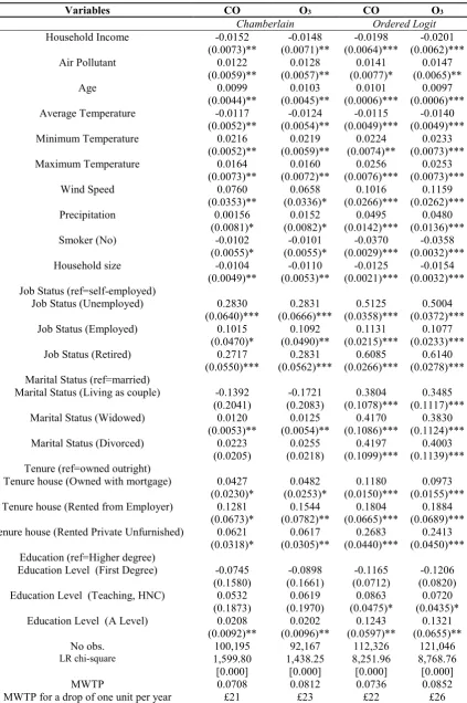
In table 4 the Chamberlain binary conditional fixed effects Logit and ordered Logit panel
regressions are reported to compare the results with those derived from the previous
approaches. The first approach gives very similar results and MWTP are very close with those
derived by adapted Probit OLS in table 2. More specifically, MWTP monetary value is £21
and £23 for CO and O3 respectively. Regarding ordered Logit the main difference is that all
the coefficients are significant indicating that all determinants are important for the health
status of individuals. However, it should be noticed that a drawback of ordered Logit
regression is that is based on random effects. The commonly used ordered probit and logit
models to identify equation (12), might lead to biased results in the coefficients of the health
status determinants, which is caused by ignoring time-invariant individual factors. However,
the MWTP is very similar with GMM estimates and it is £22 and £26 for CO and O3
respectively.
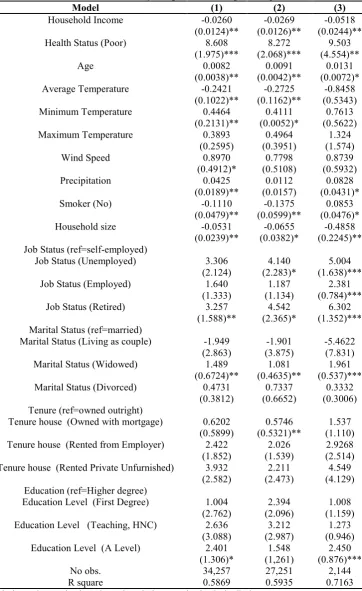
In table 5 the latent class ordered probit regressions for the CO and O3 respectively are
presented. Using conventional fixed or random effects corrects for intercept heterogeneity.
However, latent class models allow the parameters of the unobserved (latent) individual
utility function to differ across individuals i.e. slope heterogeneity (Tinbergen 1991; Clark et
al. 2005). Based on the results of table 5 it becomes clear that both air pollutants have
26
MWTP is increased in class 4 (poor health status) followed by class 3 (fair health status),
while the lowest values of MWTP are observed in classes 1 (excellent health status) and 2
(good health status). The latent class models allow for slope heterogeneity; therefore it is
possible to examine for differences of air pollution and income effects on health. Thus
different MWTP are assigned in each class. The results indicate that the respondents with
poorer health status are willing to pay more-for a drop in a unit of air pollution-than the
respondents with good self-assessed health status. It should be noticed that the MWTP in
each case is calculated based on income in every class. Additionally, the membership of class
1 is 22.87 per cent while the memberships for classes 2-4 are 45.61, 21.28 and 7.9 per cent
respectively. Age is not homogenous in health status groups as it becomes more important
factor for those with poor self reported health status. Similarly smoking becomes more
important as long as the respondents’ health status is declined. Regarding the weather
variables the effects remain the same as the findings shown before. Household size has
positive effects on health status in all classes; however it seems that the effects are more
important in class 1 when the O3 is examined. The job status remains a very important factor
for the health status in all classes. Nevertheless, being unemployed, employed and retired the
health status is less than individuals who are self-employed and the effects are increased with
the individuals’ self-reported health status. Marital status is another important determinant of
health status. More specifically, based on the results of table 5 widowed and divorced
respondents are more likely to report a lower health status than the married people, but it is
only significant for the classes 2 and 3. Similarly, living as a couple implies a lower level in
health status than people who are married and it is only significant for classes 2 and 3.
Regarding tenure, individuals who responded that they own the house with mortgage or rent
by employer or rented privately unfurnished, have a lower health status than the respondents
27
degree, first undergraduate degree or with a teaching qualification is not statistically different.
Nevertheless, the health status for individuals with A level education is lower than the
respondents who earned or are in a possession of a higher degree. Overall, the results show
that O3 and CO present negative effects on health status and the MWTP for both pollutants is
very similar across various and different econometric techniques.
In table 6 the regression results for robustness checks are reported. Regarding the weekly
averages in Panel A the air pollutants present significant effects, while the effects become
insignificant when the daily air pollution levels one day prior to interview are taken into
consideration. This is expected, as the health status is an accumulative process rather than an
instantaneous, with the exception of people who suffer from specific cardiovascular diseases
and only during high polluted days, which is rather rare in UK. More over the results using
weekly averages of air pollution are almost identical with those derived using monthly
averages. Panel B presents the results for the respondents who are located within 15 and 5
kilometres from the air monitoring stations based on the IDW method. The results for 15
kilometres are almost identical with those in table 2, while as it was expected the effects of air
pollutants on health status becomes stronger and the MWTP is increased to £23 and £26 for
O3 and CO respectively. Panel C summarises the estimates for urban and rural areas. It
becomes clear that stronger effects are reported in urban areas as it was expected, based on the
MWTP, because especially O3 is the prime ingredient of smog which is observed mainly in
the urban areas. In Panel D other specifications of the air pollutants and income are examined,
as quadratic, instead of linear terms, but the coefficients of the air pollution are found to be
insignificant. On the contrary, when the quadratic term of the income is introduced into the
regressions it becomes significant. This shows that the relationship between health status and
income is rather quadratic than monotonic. More specifically the linear term of income is
28
enough to improve health status, which the latter depends on additional expenses on medical
care including therapies, medicine and visits on general and special practitioners among
others. More specifically, the turning points for O3 and CO are respectively £12,770 and
£12,517, implying that the income has a positive effect on health status after these turning
points.In panel E the estimates for male and female separately are reported. The results show
that income is more important factor for men, while the air pollutants are more important
factors for women. In addition, the MWTP for CO and men is £16 while for women is
increased at £27. Similarly the MWTP for O3 is less for men and it is equal at £22, while for
women is £28. Finally, in panels F1-F2 the estimates for various age groups are reported. The
findings support that the individuals in the age groups 25-44 and 45-64 are willing to pay
more than the other groups followed by the older aged people and the young. However, it
should be noticed that the monetary values of MWTP are not as important as MWTP are.
More specifically, based on table 8 the MWTP for example age group 65 and older and O3 is
0.0931, while the MWTP for age groups 45-64 and 25-44 are 0.0907 and 0.0825 per cent
respectively. However, in order to estimate the average MWTP monetary values the average
household income is considered. Thus the household income per month ranges between
£2,600-£2,700 for the age groups 45-64 and 25-44, while the average household income for
people 5 years old and older is roughly £1,800.
5.2 Air Pollution, Health Status and Visits to GP
In table 7 the results of Fixed Effects Model (23) are reported. The sign of the coefficients
is similar with those presented in the previous tables. More specifically, a higher household
income and size implies a reduction of in-patient days in NHS hospital. Individuals with poor
29
The number of days is increased at 9 for the movers sample. The average temperature has
positive effects on health as it has been shown previously, leading to a decrease of in-patient
days in hospital, while minimum and maxim temperature, wind speed and precipitation result
to an increase to hospitalisation days. Therefore, controlling for meteorological variables is
important as these are significant determinants of health status. Being smoker increases the
number of hospitalisation days as well as being unemployed and retired. Living as a couple or
being divorced has no difference in the hospitalisation days relatively with the married
couples. However, widowed individuals are hospital in-patients by 1 and 2 days more for the
non-movers and movers sample respectively than the married couple. Without be a rule,
widowed people are usually old age people, as retired individuals are, reflecting the
importance of age in determining the health status. More specifically, the 89 per cent of the
total sample being widowed is 60 years old and older, while only 11 per cent is less than 60
years old. Regarding house tenure individuals owing the house with mortgage present a
higher number of in-patient days in hospital than people who own out rightly the house.
Lastly, there is no difference in the number of days among individuals with different
education level, with the exception of people with A level education for the total and the
movers sample.
In table 8 the multinomial Logit model for the number of visits in GP are reported. More
specifically, classes are the following: class 2 (one or two visits), class 3 (three to five visits),
class 4 (six to ten visits) and class 5 (more than ten visits). The reference outcome is class 1
(no visit). As it was expected, individuals with poor health status (classes 4 and 5) are visiting
GP by 7 and 11 times more than people with excellent health status (class 1). Additionally,
the results show that age is an important determinant of visit GP as the coefficient are
significantly higher in classes 4 and 5 and different than the rest of the classes. Therefore, old
30
role in health status and number of visits in GP for people with poor health status. More
specifically, the coefficients for average, minimum and maximum temperature and wind
speed are significantly higher in classes 4 and 5. More over, the average temperature has no
different effects in classes 2-3 relatively to the reference class 1. In addition, there is no
difference on precipitation effects between classes 2-4 and the reference class 1, while the
precipitation coefficient becomes significant in class 5. Thus, higher levels of precipitation,
which include air pollutants, imply that precipitation is an important determinant for people
with poor health status leading to additional visits to GP increasing the costs for NHS.
Household size in all cases leads to a reduction of GP visits and its effects become
significantly stronger for poor health individuals belonging in classes 4 and 5. This is
consistent with the previous literature that that family support and size can be protective and
beneficial to people with a chronic illness and poor health (Aldwin and Greenberger, 1987;
Doornbos, 2001). Regarding the SES and specifically, the job status employed, unemployed
and retired present a higher frequency of GP visits than self-employed. The effects are
significantly higher for retired people. Concerning the marital status there is no difference
between classes 1 and 2 of living as a couple or being widowed or divorced. However, being
widowed becomes significant for classes 3-5 and being divorced becomes significant in
classes 3-4. Finally, living as a couple, in class 5, is more likely to visit more frequently GP
than in reference class 1. House tenure and specifically, renting the house from employer or
privately increases the probability of GP visits in classes 4-5. Lastly, education level show no
difference in GP visits among classes, with the exception of class 5 where individuals with A
level education are more likely to visit GP than more educated people.
In table 9 the MWTP and its monetary value for number of in-patient days in hospital GP
are presented. The relation (12) based on the results of tables 2 and 7 is used. Based on NHS
31
days is £2,749, while the cost for non-elective (unplanned) is £527 for short stays and £2,197
for long stays. In the case examined only 1 inpatient day is taken into consideration as it is
unknown from the data how many consecutively days the individual was inpatient. Therefore,
as it was mentioned before, a person with poor health status stays on average 8 days more
than a person with good health status. In the case of table 9 the possible fee of £20 per stay
proposed by Lord Warner a former Labour health minister Borland (2014) is implemented.
Using the information provided by UK Government the minimum wage in 2010 was 5.5
(https://www.gov.uk/national-minimum-wage-rates). This is a very simplified example and
minimum wage is used as the opportunity cost for being in hospital instead of working.
Moreover the fee of £20 is equivalent with almost 2.5 working hours paid in minimum hourly
wage plus the three hours scenario which might be necessary for transportation, waiting and
consultation time. Then the MWTP monetary value for a one-unit drop in CO per year is
£137, £145 and £33 for total, non-movers and movers sample respectively, while the MWTP
values for O3 are £150, £159 and £60. Even if PM is zero then the MWTP for the total sample
becomes £95 and £98 for CO and O3 respectively for a one unit decrease in air pollutants.
Based the results of table 9 a reduction of roughly 5 units in air pollutants examined will be
equal at the elective inpatient stay costs of £2,749 and 4 units for a non elective long stay.
However, this is not precise, because the number of inpatient hospital days used in the
regressions include both planned and unplanned stays and cover all the kinds of health
episodes, as car and industrial accidents among others which are not caused from air
pollution. Therefore, the estimates overestimate the effects of air pollution or in other words
the reduction of air pollution is not realistic. However, this study suggests the examination of
air pollution effects using detailed hospitalisation data. Therefore, examining the determinants
of health status and especially the air pollution can be a very useful tool for policy makers on