Predictive ability of three different estimates of “cay” to excess stock returns A comparative study South Africa & U S

Predictive ability of three different

estimates of “cay” to excess stock returns

- A comparative study South Africa U.S.

-Emara, Noha

Rutgers University

2014

Online at

https://mpra.ub.uni-muenchen.de/68684/

Predictive Ability of Three Different Estimates of “cay”

to Excess Stock Returns

- A Comparative Study South Africa & U.S. -

Noha Emara Economics Department

Rutgers University [email protected]

Abstract

The results of Lettau and Ludvigson (2001) show that Cay-LL has a significant predictive power both in the in-sample and the out-of-sample forecast of excess return. Our study departs from Lettau and Ludvigson (2001) in adding and comparing other two estimates of cay namely cay-OLS and cay-DLS besides cay-LL for forecasting excess return in both the United States and South Africa. Using quarterly data over the period 1988:1 to 2012:2, the results for the United States suggest that the three alternative measures of cay have positive significant predicting ability for the in-sample and out-of-sample forecasting models. Furthermore, and in line with the results of Lettau and Ludvigson (2001), cay-LL has the least mean squared forecasting errors. For the case of South Africa, lagged excess return and dividend yield beat the three alternative measures of cay in forecasting excess return. The results suggest that for the case of South Africa, the trend deviations of the macroeconomic variables is not a strong predictor of the excess stock returns over a treasury bill rate, and cannot account for a statistical significant variation in future excess returns.

I. INTRODUCTION

Financial economists discuss whether excess returns are actually predictable as an overarching question. The study by Campbell and Shiller (1988) tests market efficiency based on stock price indexes by exploring whether stock prices relative to dividends predict the stock’s dividend changes into the future. Through research, they find that real earnings variable is a strong predictor of future real dividend changes. They also find that the ratio of real earnings to current price of stock partially predicts forecasting stock return.

John Campbell and Gregory Mankiw (1989) were the first economists to use wealth and asset returns to determine the current level of consumption. In their paper, they find an association between the log consumption-wealth ratio and future consumption growth and the future rate of return on invested wealth. Building upon their logic, Lettau and Ludvigson (2001) add four additional assumptions for this ratio including that the ratio is held ex-ante, wealth is the sum of asset holdings and human capital, aggregate labor income also describes unobservable human capital, and log consumption is a constant multiple of nondurables and services.

Furthermore, Letau and Ludvigson (2001), argue that macroeconomic variables play a key role in forecasting excess returns. However, in contrast to Campbell and Shiller (1988), they show that the dividend price ratio does not adequately predict excess returns through the introduction of the macroeconomic variable named “cay”: the consumption wealth ratio. They study the effect of fluctuations of the consumption-wealth ratio on both the real stock returns and excess stock returns over a Treasury bill rate. The impossibility of observing the consumption wealth ratio presents a key problem with their approach. Lettau and Ludvigson provide a solution by defining cay in terms of three integrated variables: consumption, asset holdings and labor income.

Lettau and Ludvigson (2001) have shown the trend deviations of these macroeconomic variables strongly predicts the excess stock returns over a treasury bill rate, and can account for a substantial fraction of the variation in future excess returns. The variable cay reflects the assumption that aggregate consumption carries information about future returns. Brennan and Xia (2005), nevertheless, criticize the growth of the consumption-wealth ratio as a predictor. They argue that the predictive power of cay results from a “look ahead bias,” since the information in Lettau and Ludvigson (2001) study uses information unavailable at the time of trade. The cointegration of the variables, which Lettau and Ludvigson (2001) analysis relies on throughout, causes the parameters of the regression to be estimated in-sample.

predictive power. The authors consider a situation in which two forecasts of the same variable are available, raising the possibility that of a combined forecast as a weighted average of both will achieve a more valuable combined forecasting model. Harvey, Leybourne, and Newbold (1998) address this possibility by investigating the opposite—as they describe it, an individual forecast can “encompass” the other, meaning that one forecast should optimally receive the entire weight. The authors determine such an “encompassing forecast” is not robust—that few forecasts will reflect this extreme scenario—and that the joint forecast model offered by Lettau and Ludvingson (2001) merits further investigation and discussion.

Diebold and Mariano (1995) present another rubric for evaluating forecasting models. Diebold and Mariano both propose and investigate tests for the null hypothesis of no difference in accuracy between two models, a useful exercise which informs any evaluation of a forecasting model—something which is inherent to any specific study of cay estimation, particularly as it pertains to other methods of cay estimation and even more broadly to other forecasting models, such as those described in earlier research.

Clark and McCracken (1999) also aid in our evaluation of forecasting models and accuracy, again addressing the issue of forecast encompassing investigated by Harvey, Leybourne, and Newbold (1998). Clark and McCracken (1999) offer further breadth and perspective to our understanding of possible ways to appraise forecasting models, a central task in any attempt to examine the value of cay estimation as a forecasting model. McCracken (1999) offers additional help in the form of his manuscript, “Asymptotics for Out of Sample Tests of Causality,” which—as the title suggests—contributes a method of assessing forecasting models by their ability to predict testing out-of-sample.

This study presents three different ways of estimating this trend deviation in the United States and South Africa over the period 1988:1 to 2012:2. The variables are called cay-OLS, cay-DLS and cay-LL referring to estimating the macroeconomic trend deviations using the ordinary least square method, dynamic least square method, and Ludvigson and Lettau (2001) method, respectively.

This article includes the following analysis: (1) A comparison of the ability of these three variables besides other traditional variables such as lagged excess return, dividend ratio, and payout ratio to predict in-sample excess stock return over Treasury bill rate in both South Africa and U.S. (2) An estimation of the out-of sample forecast of cay-OLS, cay-DLS and cay-LL using recursive estimation scheme for the period 2002:1 to 2012:1 for both countries. (3) A test of the ability of the unrestricted model (the one includes the variable cay) to hold all the information contained by the restricted model, or “encompass” the restricted model, using the mean squared error (MSE) F-test. (4) A comparison of the out-of sample forecast of alternative nested models using the McCracken (1999) test. (5) A test of the equivalence accuracy of two non-nested models under comparison using the Diebold and Mariano (1995) test.

forecasting regression. Section V explains Out-of-Sample Non-Nested forecasting regression. Section VI concludes the analysis of the different estimates of cay using the three different methodologies for the two countries.

II - Data:

The estimation reflects quarterly, seasonally adjusted, per capita variables, over the period of the first quarter 1988 to the first quarter of 2012 for the United States and South Africa. Consumption data here refers to non-durables consumption and services; this stock market capitalization data provides a proxy for asset wealth in both countries. Finally the data for gross national income serves as a proxy for labor income. All the data for South Africa and the United States have been collected from the databases of the “Global Finance” and “International Financial Statistics.”

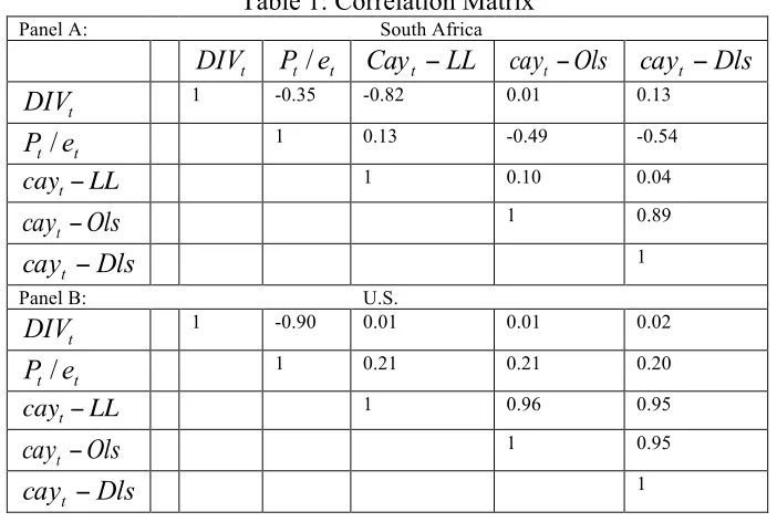
Table 1: Correlation Matrix

Panel A: South Africa

1 -0.35 -0.82 0.01 0.13

1 0.13 -0.49 -0.54

1 0.10 0.04

1 0.89

1

Panel B: U.S.

1 -0.90 0.01 0.01 0.02

1 0.21 0.21 0.20

1 0.96 0.95

1 0.95

1

Table (1) presents the correlation matrix between the financial quarterly data including the three different estimates of “cay.” Panel A shows the correlation matrix in South Africa, while panel B shows the corresponding values in the United States. This table shows the positive correlation between the three estimates of cay and the excess return for both South Africa and the United States However, the United States shows a much higher estimated correlation for the three different methods of cay.

I- Three ways of estimating the Trend Relationship Among Consumption, Labor Income and Asset Holdings;

Lettau and Ludvigson (2001) showed that can be a good proxy for market expectations of future asset returns as long as expected future returns on human capital and consumption growth are not too volatile, or as long as these variables correlate strongly with expected returns on assets. All the terms on the right-hand side of equation

t

DIV P_t /e_{t Cay LL}

t − cayt−Ols cayt −Dls

t

DIV

t t e

P/

cay_t−LL

Ols cay_t−

Dls cay_t −

t

DIV

t t e

P/

cay_t−LL

Ols cay_t−

Dls cay_t −

(1) are presumed stationary such that are cointegrated, and the left side of

(1) gives the deviation in the common trend of . This trend deviation term

will be denoted as .

(1)

In this study we will present three different ways of estimating this trend deviation. A description of the estimation follows.

Method 1: dynamic least squares (DLS) technique

The first method used to estimate the term cay is the DLS. This method follows a single equation taking this form:

(2)

where denotes the first difference operator.

This method generates optimal estimates of the cointegrating parameters in a multivariate setting. The DLS specification adds leads and lags of the first difference to the right-hand side variables to a standard OLS regression of consumption on labor income and asset holdings to eliminate the effects of the regressor endogeneity on the distribution of the least square estimator. The residual of equation (2) will be the estimated trend deviation, denoted as cay-DLS.

Method 2: Ordinary Least Square (OLS) Technique

The second method of estimating the trend deviations is the OLS. This method estimatesEquation (2) with only the lags of asset wealth and labor income included. cay is then serves as the residual of the significant regression. The cay under this second method will be denoted as cay-OLS.

Method 3: Lettau and Ludvigson (2001) Technique

This method estimates cay following the method of Lettau and Ludvigson (2001). In their paper, they estimate cay by the dynamic least square technique as in equation (2), taking the coefficients of asset wealth and labor income of the significant regression.1 cay is then calculated as follows:

(3) The estimated cay under this method will be denoted as cay-LL.

The point estimates for the parameters of consumption, labor income and assets for South Africa is

1 _{The significant regression was chosen based on the AIC measure.}

c_t,a_t, and y_t

t t t a y c , ,

t t

t a y

c −ω −(1−ω) cay_t

t i t i t h i t a i i t t t

t a y E r r c z

c (1 ) {[ _, (1 ) _, ] } (1 )

1 ω ω ω ρ ω

ω − − = _ω + − −Δ + −

− + + + ∞ =

∑

∑

∑

n a y b a b y

c , α β β , , ε

Δ t y t a t

n a y

c y

(2) (56.19) (3.22) (47.87)

and the point estimates for the equivalent model for the United States is

(3)

(-7.3) (3.5) (37.18)

where the t-statistics appear in parentheses below the coefficient estimates.

III- Quarterly In-Sample Forecasting Regressions

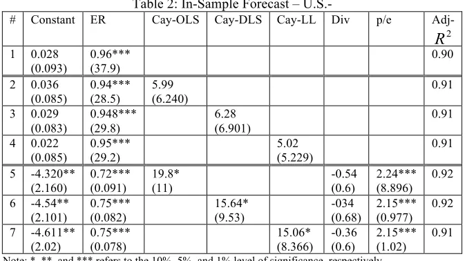
This section presents estimates of the forecasting power of different variables for the quarterly excess stock return. Table (2) presents the in-sample forecast of the U.S. excess stock return. Again the AR(1) model presented in regression one shows a statistical significant ability to predict excess stock return. Adding the different estimates of cay, regressions five through seven, slightly improves the significance of the model, but the three different estimates of cay are not statistically significant.

Adding dividends yield and payout ratio to the model, as shown in regression five through seven, the three alternative measures of cay, cay-OLS, cay-DLS, and cay-LL, show an expected positive statistical significant effect on excess return. The cay-DLS is also positive but only significant at the 15 percent level of significance. As expected, the signs of the alternative measures of cay where the deviations in the long-term trend among consumption, income, and asset holdings positively relate to future stock return. Furthermore, dividends yield shows an insignificant impact on excess return while the payout ratio was expectedly positive and statistically significant.

Table 2: In-Sample Forecast – U.S.-

# Constant ER Cay-OLS Cay-DLS Cay-LL Div p/e Adj-

1 0.028

(0.093)

0.96*** (37.9)

0.90

2 0.036

(0.085) 0.94*** (28.5) 5.99 (6.240) 0.91

3 0.029

(0.083) 0.948*** (29.8) 6.28 (6.901) 0.91

4 0.022

(0.085) 0.95*** (29.2) 5.02 (5.229) 0.91

5 -4.320**

(2.160) 0.72*** (0.091) 19.8* (11) -0.54 (0.6) 2.24*** (8.896) 0.92

6 -4.54**

(2.101) 0.75*** (0.082) 15.64* (9.53) -034 (0.68) 2.15*** (0.977) 0.92

7 -4.611**

(2.02) 0.75*** (0.078) 15.06* (8.366) -0.36 (0.6) 2.15*** (1.02) 0.91

Note: *, **, and *** refers to the 10%, 5%, and 1% level of significance, respectively.

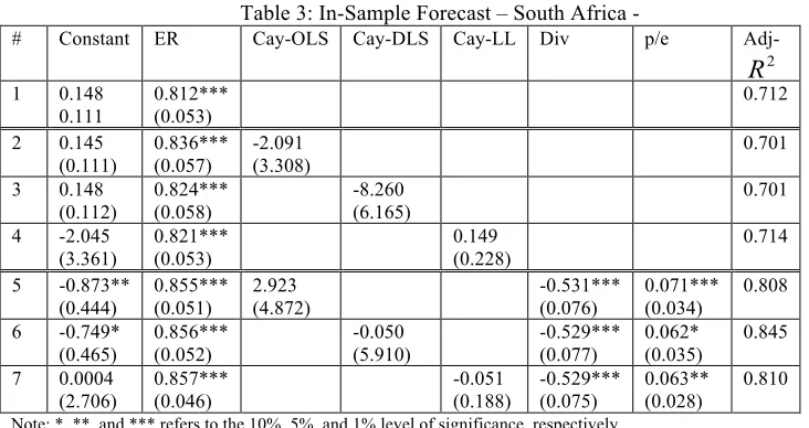
Similarly, Table (3) reports estimates from OLS regressions of excess stock returns on lagged values for the different estimates of cay and financial variable in South Africa. The regression results suggest a statistically significant AR(1) model for excess

c_n,t=3.241+0.021at+0.586yt

yt a

cn,t =−3.628+0.015 t +01.150

2

stock return in South Africa. Adding the three different estimates of cay, rows 2 through 4, does not show an improvement in the explanation of the model.

Table 3: In-Sample Forecast – South Africa -

# Constant ER Cay-OLS Cay-DLS Cay-LL Div p/e

Adj-1 0.148

0.111

0.812*** (0.053)

0.712

2 0.145

(0.111) 0.836*** (0.057) -2.091 (3.308) 0.701

3 0.148

(0.112) 0.824*** (0.058) -8.260 (6.165) 0.701

4 -2.045

(3.361) 0.821*** (0.053) 0.149 (0.228) 0.714

5 -0.873**

(0.444) 0.855*** (0.051) 2.923 (4.872) -0.531*** (0.076) 0.071*** (0.034) 0.808

6 -0.749*

(0.465) 0.856*** (0.052) -0.050 (5.910) -0.529*** (0.077) 0.062* (0.035) 0.845

7 0.0004

(2.706) 0.857*** (0.046) -0.051 (0.188) -0.529*** (0.075) 0.063** (0.028) 0.810

Note: *, **, and *** refers to the 10%, 5%, and 1% level of significance, respectively.

On the other hand, adding the financial variables represented by dividends yield and payout ratio in regressions 5-7 increases the explanation of the model. It also shows a positive, statistically significant impact of financial variables in predicting excess return. Again, the three estimates of cay do not predict excess return with statistical significance.

IV. Out-of-Sample Nested forecasting regression

The results of the in-sample forecast, especially the case of South Africa, imply that the three estimates of cay do not significantly predict excess stock return over the treasury-bill return. However, a possible estimation bias arises from the fact that these estimates of cay use the coefficient of the whole sample. An alternative model using an out-of-sample nested forecast eliminates this. The sample is split into two subsamples, an in-sample period that starts from the first quarter of 1988 to the fourth quarter of 2001 and an out-of-sample that starts from the first quarter of 2002 to the first quarter of 2012.

Using recursive estimation scheme, the analysis below compares nested forecast models based on the mean-squared forecasting error from an unrestricted model, including the three estimates of cay each one in a turn, to a restricted benchmark model. Two alternative benchmark models, a constant and a random walk, cause the unrestricted model to nest the benchmark model.

Table (4) below presents the mean squared forecast errors for nested models using alternative benchmark models. Panel A of the table presents the results for the restricted model containing the constant expected returns as the only explanatory variable and the unrestricted model containing the alternative estimates of cay besides the constant term. The results suggest that, with the exception of cay-OLS, the mean squared forecast error

2

of the other two estimates cay exceed the constant benchmark. This result applies for both South Africa and the United States.

Similarly, panel B of the same table presents the mean squared forecast error for the random walk benchmark with the three alternative estimates for cay. For the case of South Africa, the three different estimates of cay produce mean squared forecast error higher than the random walk benchmark. On the other hand, for the case of the United States the unrestricted Cay-DLS model shows the least when compared with the other two alternative estimates for cay.

Table 4: Mean Squared Forecast Errors – Nested Models Panel A

Benchmark Unrestricted Models

Constant Cay-OLS Cay-DLS Cay-LL United

States

0.212 0.211 0.215 0.214

South Africa

0.276 0.245 0.279 0.315

Panel B

Benchmark Unrestricted Models

Random walk Cay-OLS Cay-DLS Cay-LL United

States

0.236 0.240 0.263 0.218

South Africa

0.1025 0.112 0.106 0.112

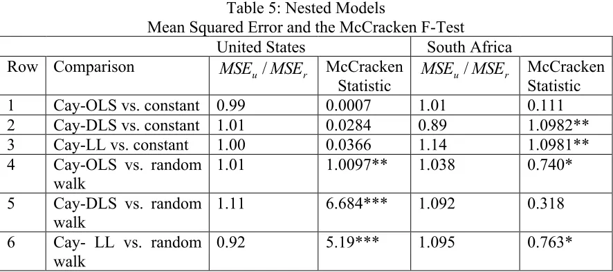
To formally compare between models, Table (5) reports the McCracken (1999) nested out-of sample F-test, or MC from here onwards, with a null hypothesis of equal predictive accuracy for the restricted and the unrestricted models. The calculated test statistics is compared with the tabulated values for recursive scheme provided by McCracken (1999).2

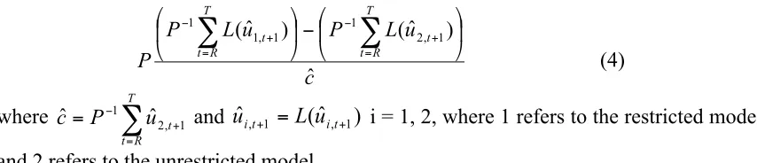
The F-test is calculated as follows

(4)

where and i = 1, 2, where 1 refers to the restricted model

and 2 refers to the unrestricted model.

The results for the United States suggest that the three alternative estimates of cay do not significantly beat the constant benchmark model. Using the random walk as the

2 _{Table (1) of McCracken (1999)}

c u L P u L P P T R t t T R t t ˆ ) ˆ ( ) ˆ

( _{1, 1} 1 _{2, 1}

1 _⎟ ⎠ ⎞ ⎜ ⎝ ⎛ − ⎟ ⎠ ⎞ ⎜ ⎝ ⎛

∑

∑

∑

benchmark model, the cay-LL beats the random walk model. The other two alternative estimates of cay, cay-OLS and cay-DLS, show a higher mean squared error than the restricted random walk model. The results of the random walk benchmark confirm the findings for the significance cay-OLS and cay-LL for the in-sample forecast for excess return. Only when compared with the random benchmark model are nested models that include cay-OLS, cay-DLS or cay-LL significant.

Table 5: Nested Models

Mean Squared Error and the McCracken F-Test

United States South Africa Row Comparison MSE_u /MSE_{r McCracken}

Statistic

r

u MSE

MSE / _McCracken

Statistic 1 Cay-OLS vs. constant 0.99 0.0007 1.01 0.111 2 Cay-DLS vs. constant 1.01 0.0284 0.89 1.0982** 3 Cay-LL vs. constant 1.00 0.0366 1.14 1.0981** 4 Cay-OLS vs. random

walk

1.01 1.0097** 1.038 0.740*

5 Cay-DLS vs. random walk

1.11 6.684*** 1.092 0.318

6 Cay- LL vs. random walk

0.92 5.19*** 1.095 0.763*

Note: *, **, and *** refers to the 10%, 5%, and 1% level of significance, respectively.

On the other hand, using the constant benchmark, the results of South Africa suggest that cay-DLS beats the constant benchmark with a statistically significant MC test statistic. The cay-OLS is, however, not statistically significant while the cay-LL does not beat the constant benchmark. In addition, using the random walk benchmark, the mean squared forecast errors of the models including the three alternative measures of cay are higher than the benchmark model. This means that the three measures of cay have less predictive ability to forecast excess return over the benchmark model. The MC test confirms these results for all models except the cay-DLS versus the random walk model.

It is worth noting that, despite the fact that none of the three alternative measures of cay show any statistically significant in-sample predictions for excess returns for the case of South Africa, using the random walk excess return as the benchmark model shows a statistically significant impact for the out-of-sample forecast.

V. Out-of-Sample Non-Nested forecasting regression

sole predictive variable of either the lagged excess return, lagged dividend yield, or lagged payout ratio.

Using the Diebold and Mariano (DM) test for out-of-sample forecast of equal predictive accuracy of two non-nested model. The null under DM test is as follows,

where 𝑔 𝜀_!! _{refers to the quadratic loss function of model i, such that 1 refers to the} restricted model and 2 refers to the unrestricted model.

Under the null hypothesis of equal predictive ability, the DM test has an asymptotically standard normal distribution and is calculated as follows3

where 𝑑!!! =𝑔 𝜀!!!! −𝑔 𝜀!!!! and the equation 𝑑 = ! 𝑑!!! 𝑃 represents the

sample estimate of _𝐸 𝑔 𝜀_!! _−𝑔 𝜀_!! _.

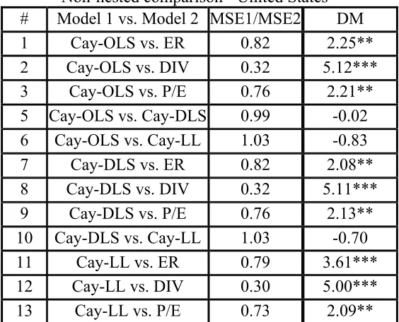
Table (6) reports the results of the DM test statistic for the out-of-sample forecast of thirteen competing non-nested models for the United States. As the results of rows 1 through 3 show, cay-OLS significantly beats the three different financial variables in predicting excess return.

Table 6: Diebold and Mariano Test Nonnested comparison United States -# Model 1 vs. Model 2 MSE1/MSE2 DM 1 Cay-OLS vs. ER 0.82 2.25** 2 Cay-OLS vs. DIV 0.32 5.12*** 3 Cay-OLS vs. P/E 0.76 2.21** 5 Cay-OLS vs. Cay-DLS 0.99 -0.02 6 Cay-OLS vs. Cay-LL 1.03 -0.83 7 Cay-DLS vs. ER 0.82 2.08** 8 Cay-DLS vs. DIV 0.32 5.11*** 9 Cay-DLS vs. P/E 0.76 2.13** 10 Cay-DLS vs. Cay-LL 1.03 -0.70 11 Cay-LL vs. ER 0.79 3.61*** 12 Cay-LL vs. DIV 0.30 5.00*** 13 Cay-LL vs. P/E 0.73 2.09**

Note: *, **, and *** refers to the 10%, 5%, and 1% level of significance, respectively.

3 _{more details are available in the paper Diebold (1995)}

0 )) ( ) ( (

: 1 2

0 E g t −g t =

H ε ε

0 )) ( ) ( (

: _t1 − _t2 ≠

A E g g

H ε ε

p T h R t h t h t p t t p t t p p g g P d P P d P d P d σ ε ε σ σ σ ˆ )) ˆ ( ) ˆ ( ( ˆ ˆ ˆ ) ( ˆ 1 1 2 1 2 / 1 1 2 / 1 1 2 / 1 2 /

1

∑

∑

∑

For example, row 1 shows that the mean squared forecast error of the regression including cay-OLS as the sole predictor for excess return is smaller than the mean square forecast error of an AR(1) model. This result is significant at the 5 percent level of significance. Similarly, rows 7 though 9 confirm that cay-DLS better predicts financial variables, and again the results were statistically significant. Finally, and in line with Lettau and Ludvigson (2001), rows 11 through 13 show that Cay-LL significantly beats ability of financial variables to predict excess stock return.

Comparing the predictive ability of the three alternative estimates of cay, the results of row 5 could not confirm the statistical significance of the better predicting ability of the cay-OLS over cay-DLS. Furthermore, the results of rows 6 and 10 could not confirm that cay-OLS and cay-DLS better forecast excess return when compared with Cay-LL. Finally, comparing the relative mean squared forecast errors of the 13 competing models, cay-LL has the least predictive errors when compared the two other estimates of cay and the three financial variables.

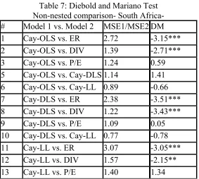
Similarly, Table (7) shows the non-nested comparison of the thirteen models in South Africa. As the results show, the predictive ability of the three alternative measures of cay could not beat the predictive ability of the lagged excess reserves or the dividends ratio. The results of rows 1, 7, and 11 show that cay-OLS, cay-DLS, and cay-LL, respectively, have a higher mean squared forecast error than the random walk benchmark model. The Diebold and Mariano test confirm the significance of this result by rejecting the null of equal predictive accuracy between the model using a measure of cay and a model using the random walk to predict excess stock return.

Table 7: Diebold and Mariano Test Non-nested comparison- South Africa- # Model 1 vs. Model 2 MSE1/MSE2 DM 1 Cay-OLS vs. ER 2.72 -3.15*** 2 Cay-OLS vs. DIV 1.39 -2.71*** 3 Cay-OLS vs. P/E 1.24 0.59 5 Cay-OLS vs. Cay-DLS 1.14 1.41 6 Cay-OLS vs. Cay-LL 0.89 -0.66 7 Cay-DLS vs. ER 2.38 -3.51*** 8 Cay-DLS vs. DIV 1.22 -3.43*** 9 Cay-DLS vs. P/E 1.09 0.05 10 Cay-DLS vs. Cay-LL 0.77 -0.78 11 Cay-LL vs. ER 3.07 -3.05*** 12 Cay-LL vs. DIV 1.57 -2.15** 13 Cay-LL vs. P/E 1.40 1.34

Note: *, **, and *** refers to the 10%, 5%, and 1% level of significance, respectively.

the model that uses the dividends ratio as the sole predictor of excess return. Again, the DM test confirms that the null hypothesis is rejected and that the competing models do not have equal predictive accuracy.

Unlike the U.S. results, as shown in rows 5, 6, and 10, in South Africa the null hypothesis of equal predictive accuracy between the three different methods of estimating cay is rejected. The results also suggest that, unlike for the United States, the null hypothesis of equal predictive accuracy between the three alternative measures of cay (rows 3, 9, and 13) and the payout ratio cannot be rejected.

VI- Conclusion

The results of Lettau and Ludvigson (2001) show that Cay-LL has a significant predictive power both in the in-sample and in the out-of-sample forecast of excess stock return. Our study departs from Lettau and Ludvigson (2001) in adding and comparing two other estimates of cay, namely cay-OLS and cay-DLS, besides cay-LL in forecasting excess return in both the United States and South Africa over the period 1988:1 to 2012:1.

Our results show that for the case of the United States, for the in sample forecast, the three alternative measures of cay show a positive statistical significant impact in predicting excess stock return. In addition, the magnitude of the effect was similar in each case. Furthermore, using out-of-sample forecast nested models with a constant benchmark, the results shows that the three alternative measures of cay could not significantly predict the excess stock return. However, using the random walk model as the benchmark, the results of the McCracken (1990) test statistic suggest that the three measures of cay do not have equal predictive accuracy with the benchmark model. However, and in line with Lettau and Ludvigson (2001), cay-LL has the least mean squared forecasting errors. In addition, using the out-of-sample non-nested models comparisons, the results of the Diebold and Mariano (1995) test show that the three measures of cay beat the financial variables, and, again, cay-LL has the least mean squared errors.

On the other hand, our results also show that for the case of South Africa, the three estimates of cay are statistically insignificant in the in-sample forecast of excess stock return. Using the constant benchmark with out-of-sample nested models comparisons, cay-DLS is the only measure of cay that significantly beats the benchmark model. In addition, using the random walk model as the benchmark model, both mean squared errors of the two models including cay-OLS and cay-LL are higher than the benchmark model. This result is confirmed by the statistically significant McCracken (1990) test. Furthermore, the out-of-sample forecast of the non-nested models shows that the lagged excess reserves and the dividend yield beat the three alternative measures of cay for predicting excess stock return. The Dieblod Mariano (1995) confirms this result.

VII- Reference:

Campbell, John Y., and Cochrane, John H., 1999. By Force of Habit: A consumption Based Explanation of Aggregate Stock Market Behavior, J.P.E 107, 205-51.

Campbell, J. Y., and R. J. Shiller, 1988. The Dividend-Price Ratio and Expectations of Future Dividends and Discount Factors, Review of Financial Studies, 1, 195-227.

Campbell, John, and N. Gregory Mankiw, 1989. Consumption, Income and Interest Rates: Reinterpreting the Time Series Evidence, National Bureau of Economic Research 4 (1989): 185-246. Print.

Clark, Todd and Michael McCracken, 1999. Tests of Equal Forecast Accuracy and encompassing for nested models, Working paper, Federal Reserve Bank of Kansas City.

Diebold, F.X. and R. Mariano, 1995. Comparing Predictive Accuracy, Journal of Business and Economic Statistics, 13, 253-3263.

Harvey, David, Stephen Leybourne, and Paul Newbold, 1998. Tests for Forecast Encompassing, Journal of Business and Economic Statistics 16,254-259.

Lettau, Martin, and Ludvigson, Sydney, 2001. Consumption, Aggregate Wealth, and Expected Stock Returns, J. Finance 56, 815-49.

Michael W. McCracken, 1999. Asymptotics for out of Sample Tests of Causality, Unpublished manuscript, Louisiana State University.