Capital Skill Complementarity: Does capital disaggregation matter?

Munich Personal RePEc Archive

Capital-Skill Complementarity: Does

capital disaggregation matter?

Correa, Juan and Lorca, Miguel and Parro, Francisco

Universidad Andres Bello, Universidad de Chile, Universidad Adolfo

Ibanez

March 2014

Capital-Skill Complementarity:

Does capital disaggregation matter?

∗

Juan A. Correa

Miguel Lorca

Francisco Parro

Abstract

Using Chilean manufacturing plants data, we find: (1) the elasticity of substitution between capital and skilled labor is lower than the elasticity of substitution between capital and unskilled labor, and (2) the higher the technological component of the capital stock the larger the size of complementarity between capital and skilled la-bor. Our findings show that capital, as an aggregate input, may under(over) state the complementarity between labor and the type of capital these workers actually use.

Keywords: capital-skill complementarity, technological capital, translog function

JEL Classification: D24, J24, L60

I. Introduction

Since Griliches (1969) first stated that capital is less substitutable for skilled labor than for unskilled labor, several studies have attempted to test this hypothesis. Although some of the literature on this topic supports the Griliches (1969) hypothesis, the evidence has been almost exclusively concentrated in developed countries. Additionally, since most of the related articles regard capital as an aggregate input and do not consider that there are also differences in the complexity of capital, they may under(over)state the complementarity between skilled labor and the type of capital that these workers actually use.

∗_{We would like to thank Roberto ´Alvarez, H´ector Calvo, Rodrigo Cerda, Edward E. Leamer, Mauricio} Larra´ın, Alejandro Micco, Carmine Ornaghi, Fernando Parro, Salvador Vald´es, Bernardita Vial, and all participants at the Chilean Ministry of Finance, Pontificia Universidad Cat´olica de Chile, and Universidad de Chile workshops, for their useful comments and suggestions. J.A. Correa also thanks FONDECYT for financial support (Grant No. 11121620).

†_{Facultad de Econom´ıa y Negocios, Universidad Andr´es Bello; Santiago, Chile, e-mail address:} jlcorrea [email protected].

This paper presents an input function model with skilled labor, unskilled labor, tech-nological capital, and non-techtech-nological capital as production factors. Using panel data from Chilean manufacturing plants, we disaggregate the stock of capital, defining three different specifications for the technological stock of capital. We find that the elasticity of substitution between capital and skilled labor is lower than the elasticity of substitu-tion between capital and unskilled labor, supporting the Griliches (1969) hypothesis in a developing country.

We also find that the higher the technological component of the capital stock the larger the size of complementarity between capital and skilled labor. Our result suggests that as the composition of the stock of capital moves toward more technological capital, the expected rise in the skill premium might be higher. This issue has generally been over-looked by the existing literature. However, our finding is important since this literature may understate the impact of capital-skill complementarity on the skill premium in coun-tries where the accumulation of technological capital is increasing rapidly. Indeed, Bruno et al. (2009) show that developing countries accumulate physical capital first and then they begin to import technological capital in a second stage of development.

Additionally, in most of our specifications, the elasticity of substitution between non-technological capital and skilled labor is larger than the elasticity of substitution between technological capital and unskilled labor; e.g., a machine can more easily substitute for skilled workers than can software for unskilled workers. We denote this result as the compensation effect, since it abates the unskilled labor demand decrease produced by the capital accumulation when capital-skill complementarity holds.

A. Related literature

Capital-skill complementarity has been extensively analyzed for developed countries.1

Nevertheless, there have been very few attempts, such as Yasar and Paul (2008) and Akay and Yuksel (2009), to verify whether the capital-skill complementarity hypothesis holds for developing countries.

Krusell et al. (2000) find that the elasticity of substitution between capital equipment and unskilled labor is higher than the elasticity of substitution between capital equipment and skilled labor. Using U.S. time series between 1963 and 1992,2 _{they find positive}

elas-ticity of substitution between capital equipment and labor for both skilled and unskilled labor; however, the estimated elasticity of substitution between capital and unskilled la-bor is around 2.5 times that of capital and skilled lala-bor. These results, though, have been criticized by Polgreen and Silos (2008), who state that the elasticity of substitution between capital equipment and unskilled labor is understated, as Krusell et al. (2000) use a capital growth that “implies very rapid growth in the stock of capital equipment.”

Using a panel of countries, Duffy et al. (2004) find weak evidence of capital-skill com-plementarity. In some of their specifications, they even find the surprising result that the hypothesis of capital-skill complementarity is more sustainable with lower thresholds for the definition of skilled labor.3

Papageorgiou and Chmelarova (2005) find no evidence of capital-skill complementarity in OECD countries. They state that capital-skill complementarity is relatively more pronounced in countries with an initial medium income and a low literacy rate. They use school attainment to construct the skilled and unskilled labor variables.

Bartel et al. (2007) posit that IT machines require operators with engineering, pro-gramming, and problem-solving skills. Therefore, technological capital is related more to specific skills than to school attainment. This point is consistent with Krueger (1993) and Autor et al. (2006), who find that computerization has increased the wages of workers who perform non-routine tasks relative to the wages of workers whose jobs involve routine tasks.4

Goldin and Katz (1998) argue that capital-skill complementarity may hold for some industries but not for others. Bergstrom and Panas (1992), using a panel of Swedish manufacturing industries, find that capital-skill complementarity holds most of the time.

1

See, for instance, Bergstrom and Panas (1992) and Krusell et al. (2000).

2

Krusell et al. (2000) construct the stock of capital using Gordon (1990) data.

3

Duffy et al. (2004) work with five thresholds to define skilled labor: (1) “workers who have attained some postsecondary education,” (2) “workers who have completed secondary education,” (3) “workers who have attained some secondary education,” (4) “workers who have completed primary education,” and (5) “workers who have attained some primary education.”

4

However, the size of capital-skill complementarity that they find is different across indus-tries.

Data sets from undeveloped economies lack of information on disaggregated measures of capital; e.g., software and computers. Akay and Yuksel (2009), for instance, define machines, tools, and other equipment as capital stock. Using panel data from Ghanaian manufacturing firms, they find that the elasticity of substitution between capital and unskilled labor is slightly higher than the elasticity of substitution between capital and skilled labor. This evidence of capital-skill complementarity in Ghana is weaker than that found by Krusell et al. (2000).

If we take into account non-technological capital only, our findings show a similar result to that found by Akay and Yuksel (2009).5 _{However, when we consider technological}

capital, our results suggest strong evidence of capital-skill complementarity, supporting the idea that the composition of capital matters. We even find that technological capital and skilled labor are complements in some specifications.

The existence of capital-skill complementarity has also been studied in international trade literature. Traditional trade theories predict that as economies open to interna-tional trade, developed countries will specialize in the production of goods that are inten-sive in skilled labor, while developing countries will produce goods that are inteninten-sive in unskilled labor. This prediction implies that the relative wage of skilled workers should increase in developed countries but decrease in developing countries as economies open to international trade.

However, the opposite phenomenon is observed in the data. As documented by Parro (forthcoming), the skill premium has increased in several developing countries. Gallego (2011) shows that the rise in the skill premium has also been present in the Chilean labor market. The latter contradicts the main prediction of the standard Heckscher-Ohlin model of trade. Therefore, it is difficult to reconcile the observed rise in the skill premium with the trade liberalization that most developing countries have experienced during recent decades.

Nevertheless, when capital-skill complementarity exists, there is an additional force balancing the effect of the Stolper-Samuelson theorem. Trade openness may stimulate investment in a developing country that opens its economy, since an important portion of equipment in that country must be imported rather than be produced by the country’s own technology (e.g., computers). Therefore, if the capital-skill complementarity hypoth-esis holds, trade openness may increase the relative demand for more educated workers and push the skill premium up in those economies. For instance, Parro (forthcoming) shows evidence that the introduction of trade in capital goods, together with capital-skill complementarity, generates a skill-biased trade effect and thus allows the possibility of an

5

important positive effect on the skill premium.

The rest of the paper is organized as follows. Section II. presents the econometric model and the construction of the elasticities of substitution. Section III. describes the data that we are working with. Section IV. shows our results and a check of robustness supporting the evidence of capital-skill complementarity and the compensation effect in most of our specifications. Section V. concludes.

II. Econometric Model

A. Translog input function

In order to answer our main question, we have to estimate the elasticities of substitution between the different labor and capital categories.

We first define a constant returns to scale and Hicks-neutral input functionF(L, S, T, K), where L denotes the working hours of unskilled workers, S the working hours of skilled workers, T technological capital, and K non-technological capital. Following Berndt and Christensen (1973) and Berndt and Christensen (1974), we assume that we can charac-terize the input function in a translog form as

lnF = β0+βLlnL+βSlnS+βT lnT +βKlnK +

1

2γLL(lnL)

2_+γLSlnLlnS

+γLT lnLlnT +γLKlnLlnK+1

2γSS(lnS)

2_{+γST lnSlnT +γSKlnSlnK}

+1

2γT T(lnT)

2_{+γT KlnTlnK+} 1

2γKK(lnK)

2_.

We also assume that markets are competitive; thus, ∂F

∂L =PL, ∂F

∂S =PS, ∂F

∂T =PT, and ∂F

∂K =PK, wherePi denotes the price of inputirelative to the price of the aggregate input function F. Knowing that ∂_∂ln_lnF_i = Pii

F , the cost share of input i (si), we have

sL=βL+γLLlnL+γLSlnS+γLT lnT +γLKlnK,

sS =βS+γLSlnL+γSSlnS+γSTlnT +γSKlnK,

sT =βT +γLTlnL+γST lnS+γT TlnT +γT KlnK,

sK =βK+γLKlnL+γSKlnS+γT KlnT +γKKlnK.

Since the cost shares must sum up to 1, we assume the additional restrictions that γij =γji and P

inputs by K, and therefore dropping the last row and column of the system, we have the factor shares used in the estimation given by

sL =βL+γLLln L

K +γLSln S

K +γLT ln T K,

sS =βS+γLSln L

K +γSSln S

K +γSTln T

K, (1)

sT =βT +γLTln L

K +γSTln S

K +γT Tln T K.

We can now solve this system by Feasible Generalized Least Squares (FGLS),6 _defining

y′i =

sL sS sT

,

β′ =

βL γLL γLS γLT βS γSS γST βT γT T

, and Xi =     

1 ln L K ln

S K ln

T

K 0 0 0 0 0

0 0 ln_KL 0 1 ln_KS ln_KT 0 0

0 0 0 ln L

K 0 0 ln S

K 1 ln T K      .

We can estimate ˆβ as

ˆ

β = (X′(Ω⊗IN)−1_X)−1_X′_(Ω⊗IN)−1_{y, (2)}

with Ω as the variance-covariance matrix and IN an identity matrix of size N.

B. Elasticities of substitution

Once we have ˆβ, we can estimate input shares ˆsi and compute elasticities of substitution using Allen-Uzawa elasticities defined as

ˆ

σij = γijˆ + ˆsisjˆ ˆ

sisjˆ , (3)

ˆ

σii= γiiˆ + ˆsi

2_−siˆ

ˆ

si2 .

6

We then use ˆσij to test whether capital-skill complementarity holds. We define relative capital-skill complementarity as ˆσzL >σzSˆ and absolute capital-skill complementarity as ˆ

σzL >0>σzSˆ ,∀z ∈ {T, K}.

When disaggregating capital, we can also check the order of the elasticity of substitution between non-technological capital and skilled labor (ˆσKS), and the elasticity of substitu-tion between technological capital and unskilled labor (ˆσT L). If ˆσKS >σT Lˆ (ˆσKS <σT L),ˆ we can argue that a machine is more (or less) substitutable for skilled workers than soft-ware is for unskilled workers. We denote this as the compensation (or augmenting) effect.

Whenever capital-skill complementarity holds, there are two cases of analysis to check whether we have the compensation effect (ˆσKS > σT L) or the augmenting effect (ˆˆ σKS < ˆ

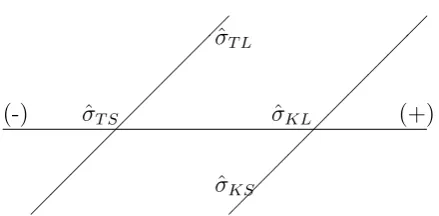
σT L). The first case assumes that ˆσT S > σKL; i.e., the elasticity of substitution be-ˆ tween technological capital and skilled labor is larger than the elasticity of substitution between non-technological capital and unskilled labor. Figure 1 shows the relative order of the elasticities of substitution, where the value increases toward the right-hand side. Although we cannot compare ˆσKS with ˆσT L directly, capital-skill complementarity im-plies that ˆσT L >σT Sˆ and ˆσKL >σKSˆ . Therefore, ˆσT L is unambiguously larger than ˆσKS (augmenting effect).

However, if we assume the second case, that ˆσT S < σKL, both effects are possible, asˆ we can see in figure 2. By capital-skill complementarity, we know that ˆσKL > σKSˆ and ˆ

σT L >σT Sˆ ; thus, the order between ˆσT L and ˆσKS is ambiguous. In this case, whether we have the compensation effect or the augmenting effect depends on the distance of ˆσKL to ˆ

σKS and to ˆσT L.

Since ˆσT S > σKLˆ means that software is more substitutable for skilled workers than machines are for unskilled workers (a case very unlikely to occur), without loss of gener-ality, our analysis focuses on the assumption that ˆσT S <σKL. Figure 3 shows isoquantsˆ of the four different input relations that we are interested in. Vertical axes denote the type of capital, while horizontal axes denote the type of labor. By capital-skill comple-mentarity, we know that ˆσKL > ˆσKS and ˆσT L > σT Sˆ . The latter is the reason why the isoquant in subfigure 3b (subfigure 3d) is more L-shaped than the isoquant in subfigure 3a (subfigure 3c). From ˆσT S <σKL, we also know that the isoquant in subfigure 3d is moreˆ L-shaped than the isoquant in subfigure 3a. What we do not know is whether the isoquant in subfigure 3b is more or less L-shaped than the isoquant in subfigure 3c.

Whenever the isoquant shape in subfigure 3a is more (less) similar to the isoquant shape in subfigure 3b than to that in subfigure 3c; i.e., ˆσKL >σKSˆ >σT Lˆ (ˆσKL >σT Lˆ > ˆ

σKS), the compensation effect (augmenting effect) holds. We can carry out the equivalent exercise stating that whenever the isoquant shape in subfigure 3d is more (less) similar to the isoquant shape in subfigure 3c than to that in subfigure 3b; i.e., ˆσT S <σT Lˆ <σKSˆ (ˆσT S <σKSˆ <σT L), the compensation effect (augmenting effect) holds.ˆ

whenever horizontal differences are smaller (larger) than vertical differences. The intuition behind this can be seen as a combination of two factors: the user-friendliness of the type of capital, which determines the level of capital-skill complementarity, and the size of the labor substitution generated by the type of capital.

It is reasonable to assume that a user-friendly machine would be used by a lower ratio of skilled to unskilled workers than a very complex machine. Therefore, the more user-friendly the capital input, the smaller the degree of capital-skill complementarity. If a process uses user-friendly machines, but these machines can perform tasks that would otherwise be performed by a large number of workers, we expect the compensation effect to hold. On the contrary, if machines are complex to use and do not substitute for too many workers, the augmenting effect is more likely to hold.

III. Data and Variables

To perform the empirical analysis, we use the Annual Chilean Survey of Manufacturers (ENIA) panel data from 2000 to 2011. Conducted by the Chilean Institute of Statistics, the ENIA is an annual census of manufacturing plants with 10 or more employees. ENIA data have been used in many relevant studies, such as Tybout et al. (1991), Liu (1993), Levinsohn (1999), Pavcnik (2002), and Levinsohn and Petrin (2003), among others.

The ENIA 2000-2011 provides us with a representative database of the Chilean man-ufacturing sector. We focus our analysis on the plants that are linked to a particular industry.7 _{Thus, we include plants operating in 52 industries identified by the}

Interna-tional Standard Industrial Classification (ISIC) at the three-digit level.8

The data retrieved from the ENIA 2000-2011 include gross fixed assets, depreciation of gross fixed assets, investment in fixed assets, labor hours, number of workers, labor compensation, value added, financial cost, corporate taxes, exports, IT expenditure, in-termediate expenditure, ownership, location, and ISIC code.

The ENIA 2000-2010 provides the previous year’s value and the current year’s invest-ment in eight types of fixed assets: land, buildings, machinery and equipinvest-ment, furniture and fixtures, vehicles, software, other tangible fixed assets, and other intangible assets.9

Using the perpetual inventory method, we can therefore compute the capital stock for each type of asset as

kit = (1−δk)kit−1+Iit,

7

We do not include plants without an ISIC industry classification or plants with negative values of

T _and/orK_{, which occurs when plants sell their fixed assets (negative investment) and the last-period}

capital stock discounted by depreciation is not large enough to compensate for the negative investment.

8

Table 1 shows the industries of our data, at the ISIC-2 level. We use the classifications provided by the third revision of the ISIC.

9

where kit is the type of fixed asset for plant i at time t, δk denotes the depreciation rate of fixed asset k,10 _{and I is the investment in fixed asset k.}11

We calculate the aggregate rental cost of capital r as

r= B+δ 1−τ,

with B as the discount rate and τ the effective corporate tax rate.12

In order to define both technological capital T and non-technological capital K, we build three different specifications. In Specification 1, we define T as software and K as the rest of fixed assets. In Specification 2, we define T as software plus intangible assets. Finally, in Specification 3, we define T as the sum of software, other intangible assets, machinery and equipment, and other tangible fixed assets.

The ENIA contains detailed information on both labor hours and labor compensation for non-specialized personnel, maintenance workers, clerks, personal service workers, spe-cialized workers, administrative personnel, and managers. We define spespe-cialized workers, administrative personnel, and managers as skilled workers S, and the rest of the cate-gories as unskilled workers L. As a crude robustness check of our definition of skilled and unskilled workers, we computed the average percentage of skilled hours over the total hours in the data set. Around 23% of the total hours corresponds to skilled labor. This number is roughly close to the fraction of workers who complete a college education in Chile.

IV. Empirical Results

We now estimate the model developed in section II. Our procedure consists first of an OLS estimation of the system equation (1) to obtain each ˆsi and their respective resid-uals. We then construct the variance-covariance matrix Ω of the residuals and take the Kronecker product of Ω and an identity matrix. After that, we compute ˆβ, determined by equation (2). We then use ˆβ to estimate ˆsi and insert them in equation (3) to obtain the Allen-Uzawa elasticities of substitution ˆσij. Finally, we compute 95% confidence intervals

10

We use a depreciation rate of 2.5%, 13%, 25%, 13%, and 31.5% for buildings, machinery and equip-ment, vehicles, intangible assets, and software, respectively, as documented by Oulton and Srinivasan (2003). We use a depreciation rate of 18% for other tangible fixed assets, as reported by the U.S. Bureau of Economic Analysis.

11

Investment is defined as the purchase of new and used assets plus asset improvements minus the sales of used assets.

12

The depreciation rateδ_{used in this formula is the weighted average of the fixed assets’ depreciation}

rates. We follow Cerda and Saravia (2009) to compute the discount rate B _{and the effective corporate}

tax rate τ_{, where} B _{is the weighted average of the ratio of financial cost to value added and} τ _{is the}

for ˆσij using the bootstrap method.13 _{All tables include results from both pooled and}

fixed effects regressions.

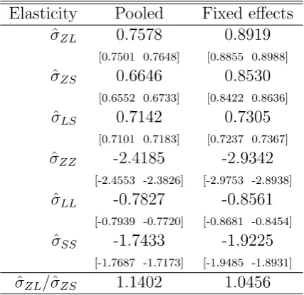
We first test capital-skill complementarity considering the aggregate level of capital; i.e., without distinguishing between technological and non-technological capital. DefiningZ = T +K, as we can see in Table 3, the elasticity of substitution between aggregate capital and skilled labor (ˆσZS) is lower than the elasticity of substitution between aggregate capital and unskilled labor (ˆσZL), denoting relative capital-skill complementarity.14 _This

result constitutes novel empirical evidence of capital-skill complementarity for a develping economy. As discussed in section I., this result is important since it allows to reconciliate the observed rise in the skill premium with the trade liberalization that most developing countries have experienced in recent decades.

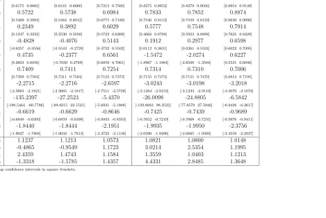
We now compare the aggregate and disaggregate elasticities of substitution, using the four specifications described in section III.. Table 5 shows the elasticities of substitution for the disaggregate specifications.15 _{We can see that there is both technological and}

non-technological capital-skill complementarity for all specifications. However, as soon as we use more disaggregate definitions of technological capital, the size of technological capital-skill complementarity (defined as |σT Lˆ −σT Sˆ |) increases, while the size of non-technological capital-skill complementarity remains roughly the same. We can even see that there is absolute technological capital-skill complementarity in Specifications 1 and 2 for the pooled regressions, whereas technological and non-technological capital-skill complementarity are very similar in Specification 3.

Another interesting result, which can be analyzed from Table 5, is that the compen-sation effect holds in all specifications (ˆσKS > ˆσT L). We can also see that as soon as we consider a more aggregate definition of technological capital, the compensation effect decreases. As both ˆσKL and ˆσKS remain roughly similar in the three specifications, what drives this result is that as soon as we consider more aggregate definitions for technolog-ical capital, ˆσT S increases faster than ˆσT L does. Therefore, the elasticity of substitution between technological capital and skilled labor is relatively more sensitive to the techno-logical level of capital.

V. Conclusion

Using data from Chilean manufacturing plants, we find that the elasticity of substitution between capital and skilled labor is lower than the elasticity of substitution between capital and unskilled labor, supporting the Griliches (1969) capital-skill complementarity hypothesis in a developing country.

13

We perform the nonparametric bootstrap method (resampling with replacement) with 1,000 replica-tions.

14

Table 2 shows the coefficients of equation (1) for the aggregate specification.

15

Additionally, we find that the technological capital-skill complementarity is significantly larger than the non-technological capital-skill complementarity, for different specifications of technological capital. That is, the higher the technological component of the capital stock the larger the size of complementarity between capital and skilled labor. Our results show that related articles regarding capital as an aggregate input, and disregarding that there are also differences in the complexity of capital, may under(over)state the complementarity between skilled labor and the type of capital that these workers actually use.

Another interesting result from our estimations is that the elasticity of substitution between non-technological capital and skilled labor is larger than the elasticity of sub-stitution between technological capital and unskilled labor. We call this phenomenon a compensation effect, since it compensates for the decrease in the unskilled labor demand when capital-skill complementarity holds. This finding may sound counterintuitive, as it suggests, for example, that software is less substitutable for unskilled workers than are machines for skilled workers. However, we show that the compensation effect may occur when the productivity of skilled workers using non-technological capital is higher but close to the productivity of unskilled workers using that kind of capital. This is in-deed the intuitive case. For instance, the productivity gap between skilled and unskilled workers driving a car or operating machines that perform routine tasks should be rela-tively small. If this is accompanied by the fact that non-technological capital substitutes for many more unskilled workers than technological capital does for skilled workers, the compensation effect is likely to hold. We find that the compensation effect is stronger when the technology level of the capital stock increases. This phenomenon occurs because the elasticity of substitution between technological capital and unskilled labor strongly decreases as soon as technological machines become more high-tech.

An interesting extension of this paper is to find the mechanism of how imports affect the skill premium. Since the composition of capital matters, an increase in technological capital imports, ceteris paribus, may raise the relative demand of skilled workers. This issue has been overlooked by the literature so far and it may help us understand not only the evolution of the skill premium over time but also cross-sectional variations of the skill premium at some moment in time.

References

Akay, G. H. and M. Yuksel (2009). Capital-skill complementarity: Evidence from manu-facturing industries in Ghana. IZA D.P. No. 4674.

Autor, D., L. F. Katz, and M. S. Kearney (2006). The polarization of the U.S. labor market. American Economic Review 96(2), 189–194.

Bartel, A., C. Ichniowski, and K. Shaw (2007). How does information technology affect productivity? plant-level comparisons of product innovation, process improvement, and worker skills. Quarterly Journal of Economics 122(4), 1721–1758.

Bergstrom, V. and E. E. Panas (1992). How robust is the capital-skill complementarity hypothesis? Review of Economics and Statistics 74(3), 540–546.

Berndt, E. R. and L. R. Christensen (1973). The internal structure of functional relation-ships: Separability, substitution, and aggregation. Review of Economic Studies 40(3), 403–410.

Berndt, E. R. and L. R. Christensen (1974). Testing for the existence of a consistent aggregate index of labor inputs. American Economic Review 64(3), 391–404.

Bruno, O., C. Le Van, and B. Masquin (2009). When does a developing country use new technologies? Economic Theory 40(2), 275–300.

Cerda, R. A. and D. Saravia (2009). Corporate tax, firm destruction and capital stock accumulation: Evidence from Chilean plants, 1979-2004. Central Bank of Chile Working Paper No. 521.

Duffy, J., C. Papageorgiou, and F. Perez-Sebastian (2004). Capital-skilll complementar-ity? evidence from a panel of countries. Review of Economics and Statistics 86(1), 327–344.

Gallego, F. (2011). Skill premium in chile: Studying skill upgrading in the south. World Development 68(1), 29–51.

Goldin, C. and L. F. Katz (1998). The origins of technology-skill complementarity. Quar-terly Journal of Economics 113(3), 693–732.

Gordon, R. J. (1990). The Measurement of Durable Goods Prices. Chicago: University of Chicago Press.

Griliches, Z. (1969). Capital-skill complementarity. Review of Economics and Statis-tics 51(4), 465–468.

Krueger, A. B. (1993). How computers have changed the wage structure: Evidence from microdata, 1984-1989. Quarterly Journal of Economics 108(1), 33–60.

Levinsohn, J. (1999). Employment responses to international liberalization in Chile. Journal of International Economics 47(2), 321–344.

Levinsohn, J. and A. Petrin (2003). Estimating production functions using inputs to control for unobservables. Review of Economic Studies 70(2), 317–341.

Liu, L. (1993). Entry-exit, learning, and productivity change evidence from Chile.Journal of Development Economics 42(2), 217–242.

Oulton, N. and S. Srinivasan (2003). Capital stocks, capital services, and depreciation: an integrated framework. Bank of England Working Paper No. 192.

Papageorgiou, C. and V. Chmelarova (2005). Nonlinearities in capital-skill complemen-tarity. Journal of Economic Growth 10(1), 59–89.

Parro, F. (Forthcoming). Capital-skill complementarity and the skill premium in a quan-titative model of trade. American Economic Journal: Macroeconomics.

Pavcnik, N. (2002). Trade liberalization, exit, and productivity improvement: Evidence from Chilean plants. Review of Economic Studies 69(1), 245–276.

Polgreen, L. A. and P. Silos (2008). Capital-skill complementarity and inequality: A sensitivity analysis. Review of Economic Dynamics 11(2), 302–313.

Tybout, J., J. de Melo, and V. Corbo (1991). The effects of trade reforms on scale and tech-nical efficiency: New evidence from Chile. Journal of International Economics 31(3-4), 231–250.

Uzawa, H. (1962). Production functions with constant elasticities of substitution. Review of Economic Studies 29(4), 291–299.

Wooldridge, J. M. (2003). Econometric Analysis of Cross Section and Panel Data. Mas-sachusetts: The MIT Press.

A Figures and Tables

(-) ˆσKL σT Sˆ (+)

ˆ σKS

ˆ σT L

Figure 1: Augmenting effect when ˆσT S >σKLˆ

(-) ˆσT S σKLˆ (+)

ˆ σT L

ˆ σKS

(a) Non-technological capital and unskilled la-bor

(b) Non-technological capital and skilled labor

(c) Technological capital and unskilled labor (d) Technological capital and skilled labor

Table 1: R&D Groups of Industries by ISIC Number

High

24 Manufacture of chemicals and chemical products 29 Manufacture of machinery and equipment n.e.c.

30 Manufacture of office, accounting and computing machinery 31 Manufacture of electrical machinery and apparatus n.e.c.

32 Manufacture of radio, television and communication equipment and apparatus 33 Manufacture of medical, precision and optical instruments, watches and clocks 34 Manufacture of motor vehicles, trailers and semi-trailers

35 - 351 Manufacture of other transport equipment except building and repairing of ships and boats

Medium

23 Manufacture of coke, refined petroleum products and nuclear fuel 25 Manufacture of rubber and plastics products

26 Manufacture of other non-metallic mineral products 27 Manufacture of basic metals

28 Manufacture of fabricated metal products, except machinery and equipment 351 Building and repairing of ships and boats

Low

15 Manufacture of food products and beverages 16 Manufacture of tobacco products

17 Manufacture of textiles

18 Manufacture of wearing apparel; dressing and dyeing of fur

19 Tanning and dressing of leather; manufacture of luggage, handbags, saddlery, harness and footwear

20 Manufacture of wood and of products of wood and cork, except furniture; manufacture of articles of straw and plaiting materials

21 Manufacture of paper and paper products

22 Publishing, printing and reproduction of recorded media 36 Manufacture of furniture; manufacturing n.e.c.

Table 2: Coefficients of Equation (1) for the Aggregate Specification

Pooled Fixed effects

Variables sL sS sL sS

Ln(L/Z) 0.0665 -0.0395 0.0493 -0.0373

(0.000346)∗∗∗ _(0.000257)∗∗∗ _(0.000329)∗∗∗ _(0.000267)∗∗∗

Ln(S/Z) -0.0395 0.0616 -0.0373 0.0470

(0.000257)∗∗∗ _(0.000299)∗∗∗ _(0.000267)∗∗∗ _(0.000295)∗∗∗

β 0.4630 0.3840 -0.0042 -0.0092

(0.00269)∗∗∗ _(0.00249)∗∗∗ _(0.00156)∗∗∗ _(0.00149)∗∗∗

Observations 33,003 33,003 33,003 33,003

R-squared 0.540 0.567 0.433 0.446

Standard errors in parentheses. ()∗∗∗_{Significant at the 1% level.}

Table 3: Elasticities of Substitution for the Aggregate Specification

Elasticity Pooled Fixed effects ˆ

σZL 0.7578 0.8919

[0.7501 0.7648] [0.8855 0.8988]

ˆ

σZS 0.6646 0.8530

[0.6552 0.6733] [0.8422 0.8636]

ˆ

σLS 0.7142 0.7305

[0.7101 0.7183] [0.7237 0.7367]

ˆ

σZZ -2.4185 -2.9342

[-2.4553 -2.3826] [-2.9753 -2.8938]

ˆ

σLL -0.7827 -0.8561

[-0.7939 -0.7720] [-0.8681 -0.8454]

ˆ

σSS -1.7433 -1.9225

[-1.7687 -1.7173] [-1.9485 -1.8931]

ˆ

σZL/ˆσZS 1.1402 1.0456

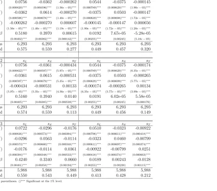
Table 4: Coefficients of Equation (1) for the Disaggregate Specifications

Pooled Fixed effects

Specification 1 sL sS sT sL sS sT

Ln(L/K) 0.0756 -0.0362 -0.000262 0.0544 -0.0375 -0.000145

(0.000820)∗∗∗ _(0.000596)∗∗∗ _(1.56e

−05)∗∗∗ (0.000789)∗∗∗ (0.000629)∗∗∗ (1.90e−05)∗∗∗

Ln(S/K) -0.0362 0.0614 -0.000270 -0.0375 0.0503 -0.000147

(0.000596)∗∗∗ _(0.000678)∗∗∗ _(1.40e

−05)∗∗∗ (0.000629)∗∗∗ (0.000698)∗∗∗ (1.72e−05)∗∗∗

Ln(T /K) -0.000262 -0.000270 0.000607 -0.000145 -0.000147 0.000656

(1.56e−05)∗∗∗ (1.40e−05)∗∗∗ (1.19e−05)∗∗∗ (1.90e−05)∗∗∗ (1.72e−05)∗∗∗ (1.20e−05)∗∗∗

β 0.5180 0.3970 0.00615 0.0192 7.67e-05 -5.28e-05

(0.00402)∗∗∗ _(0.00382)∗∗∗ _(0.000142)∗∗∗ _(0.00255)∗∗∗ _{(0.00245) (5.18e}

−05)

Observations 6,293 6,293 6,293 6,293 6,293 6,293 R-squared 0.575 0.559 0.277 0.449 0.457 0.320

Specification 2 sL sS sT sL sS sT

Ln(L/K) 0.0756 -0.0361 -0.000434 0.0544 -0.0375 -0.000174

(0.000822)∗∗∗ _(0.000597)∗∗∗ _(5.97e

−05)∗∗∗ (0.000789)∗∗∗ (0.000629)∗∗∗ (6.35e−05)∗∗∗

Ln(S/K) -0.0361 0.0615 -0.000531 -0.0375 0.0503 -0.000265

(0.000597)∗∗∗ _(0.000679)∗∗∗ _(5.35e

−05)∗∗∗ (0.000629)∗∗∗ (0.000699)∗∗∗ (5.77e−05)∗∗∗

Ln(T /K) -0.000434 -0.000531 0.00133 -0.000174 -0.000265 0.00134

(5.97e−05)∗∗∗ (5.35e−05)∗∗∗ (4.56e−05)∗∗∗ (6.35e−05)∗∗∗ (5.77e−05)∗∗∗ (3.99e−05)∗∗∗

β 0.5160 0.3940 0.0140 0.0191 6.02e-05 5.58e-05

(0.00405)∗∗∗ _(0.00385)∗∗∗ _(0.000539)∗∗∗ _(0.00255)∗∗∗ _{(0.00245) (0.000176)}

Observations 6,293 6,293 6,293 6,293 6,293 6,293 R-squared 0.574 0.559 0.113 0.449 0.456 0.149

Specification 3 sL sS sT sL sS sT

Ln(L/K) 0.0722 -0.0296 -0.0176 0.0510 -0.0323 -0.00922

(0.000826)∗∗∗ _(0.000573)∗∗∗ _(0.000394)∗∗∗ _(0.000798)∗∗∗ _(0.000611)∗∗∗ _(0.000418)∗∗∗

Ln(S/K) -0.0296 0.0563 -0.0114 -0.0323 0.0460 -0.00799

(0.000573)∗∗∗ _(0.000660)∗∗∗ _(0.000348)∗∗∗ _(0.000611)∗∗∗ _(0.000697)∗∗∗ _(0.000374)∗∗∗

Ln(T /K) -0.0176 -0.0114 0.0361 -0.00922 -0.00799 0.0251

(0.000394)∗∗∗ _(0.000348)∗∗∗ _(0.000533)∗∗∗ _(0.000418)∗∗∗ _(0.000374)∗∗∗ _(0.000663)∗∗∗

β 0.4240 0.3340 0.0660 0.0189 0.00243 -0.0128

(0.00401)∗∗∗ _(0.00358)∗∗∗ _(0.00194)∗∗∗ _(0.00255)∗∗∗ _{(0.00238) (0.00115)}∗∗∗

Observations 5,988 5,988 5,988 5,988 5,988 5,988 R-squared 0.550 0.543 0.449 0.413 0.428 0.212

Table 5: Elasticities of Substitution for the Disaggregate Specifications

Pooled Fixed effects

Elasticity Specification 1 Specification 2 Specification 3 Specification 1 Specification 2 Specification 3 ˆ

σKL 0.6430 0.6434 0.7384 0.8476 0.8480 0.9005

[0.6175 0.6662] [0.6181 0.6666] [0.7213 0.7560] [0.8275 0.8652] [0.8279 0.8656] [0.8854 0.9148]

ˆ

σKS 0.5722 0.5738 0.6984 0.7833 0.7852 0.8874

[0.5469 0.5994] [0.5484 0.6012] [0.6775 0.7180] [0.7540 0.8113] [0.7559 0.8133] [0.8639 0.9090]

ˆ

σT L 0.2349 0.3892 0.6029 0.5777 0.7548 0.7914

[0.1247 0.3232] [0.2530 0.5050] [0.5723 0.6309] [0.4668 0.6788] [0.5953 0.8898] [0.7625 0.8229]

ˆ

σT S -0.4828 -0.4076 0.5143 0.1912 0.2977 0.6598

[-0.6257 -0.3556] [-0.5543 -0.2728] [0.4732 0.5502] [0.0112 0.3631] [0.0261 0.5524] [0.6022 0.7095]

ˆ

σKT 0.4735 -0.2377 0.6561 -1.5472 -2.0274 0.6227

[0.2603 0.6856] [-0.7039 0.2769] [0.6059 0.7061] [-1.8967 -1.1884] [-2.6508 -1.3504] [0.5531 0.6946]

ˆ

σLS 0.7409 0.7411 0.7254 0.7314 0.7310 0.7006

[0.7309 0.7503] [0.7311 0.7504] [0.7123 0.7373] [0.7155 0.7473] [0.7151 0.7470] [0.6814 0.7195]

ˆ

σKK -2.2715 -2.2716 -2.6597 -3.0243 -3.0198 -3.2018

[-2.3663 -2.1821] [-2.3665 -2.1817] [-2.7511 -2.5728] [-3.1284 -2.9153] [-3.1233 -2.9110] [-3.3070 -3.1078]

ˆ

σT T -135.2397 -27.2523 -5.4370 -26.0098 -24.8805 -6.5842

[-198.5464 -60.7786] [-89.9215 22.1521] [-5.6931 -5.1908] [-129.8683 98.3522] [-77.8579 27.5946] [-6.9426 -6.2617]

ˆ

σLL -0.6619 -0.6629 -0.8646 -0.7425 -0.7439 -0.9689

[-0.6848 -0.6393] [-0.6859 -0.6398] [-0.8933 -0.8353] [-0.7652 -0.7219] [-0.7668 -0.7231] [-0.9976 -0.9411]

ˆ

σSS -1.8440 -1.8444 -2.1951 -1.9935 -1.9950 -2.3756

[-1.9027 -1.7808] [-1.9032 -1.7813] [-2.2722 -2.1138] [-2.0590 -1.9296] [-2.0605 -1.9309] [-2.4559 -2.2937]

ˆ

σKL/σˆKS 1.1237 1.1213 1.0573 1.0821 1.0800 1.0148

ˆ

σT L/σˆT S -0.4865 -0.9549 1.1723 3.0214 2.5354 1.1995

ˆ

σKS/σˆT L 2.4359 1.4743 1.1584 1.3559 1.0403 1.1213

ˆ

σ /σˆ -1.3318 -1.5785 1.4357 4.4331 2.8485 1.3648