MDSENT at SemEval 2016 Task 4: A Supervised System for Message Polarity Classification

MDSENT at SemEval-2016 Task 4: A Supervised System for Message

Polarity Classification

Hang Gao and Tim Oates

hanggao1@umbc.edu, oates@cs.umbc.edu University of Maryland Baltimore County

11000 Hilltop Circlet Baltimore, MD 21250, USA

Abstract

This paper describes our system submitted for the Sentiment Analysis in Twitter task of SemEval-2016, and specifically for the Mes-sage Polarity Classification subtask. We used a system that combines Convolutional Neural Networks and Logistic Regression for senti-ment prediction, where the former makes use of embedding features while the later utilizes various features like lexicons and dictionaries.

1 Introduction

Recently, rapid growth of the amount of user-generated content on the web prompts increasing in-terest in research on sentiment analysis and opinion mining. A typical example is Twitter, where lots of users express feelings and opinions about vari-ous subjects. However, unlike traditional media, lan-guage used in social network services like Twitter is often informal, leading to new challenges to corre-sponding text analysis.

The SemEval-2016 Sentiment Analysis in Twit-ter task (SESA-16) is a task that focuses on the sentiment analysis of tweets. As a continuation of SemEval-2015 Task 10, SESA-16 introduces sev-eral new challenges, including the replacement of classification with quantification, movement from two/three-point scale to five-point scale, etc.

We participated in Subtask A of SESA-16, namely message polarity classification, a task that seeks to predict a sentiment label for some given text. We model the problem as a multi-class classifi-cation problem that combines the predictions given by two different classifiers: one is a Convolutional

Neural Network (CNN) and the other is Logistic Re-gression (LR). The former takes embedding-based features while the latter utilizes various features such as lexicons, dictionaries, etc.

The remainder of this paper is structured as fol-lows. In Section 2, we describe our system in de-tail, including feature description and approaches. In Section 3, we list the details of datasets for the ex-periments, along with hyperparameter settings and training techniques. In Section 4, we report the ex-periment results and present the corresponding dis-cussion.

2 System Description

Our system aims at predicting the sentiment of a given message, i.e., whether the message expresses positive, negative or neutral emotion. To achieve that, we adopt two separate classifiers, CNN and LR, designed to utilize different types of features. The fi-nal prediction for sentiment is a combination of pre-dictions given by both classifiers.

2.1 Data Preprocessing

Tweets often include informal text, making it es-sential to preprocess tweets before they are fed to the system. However, we keep the preprocessing to a minimum by only removing URLs and @User tags. We then further tokenize and tag tweets with arktweetnlp (Gimpel et al., 2011). In addition, all tweets are lower-cased.

2.2 Logistic Regression

We use the LR classifier for features from sentiment lexicons and token clusters. We have used the

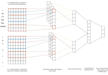
Figure 1:CNN architecture for an example with both word-based and character-based input maps.

lowing:

• clusters: 1000 token clusters provided by the

CMU tweet NLP tool. These clusters are pro-duced with the Brown clustering algorithm on 56 million English-language tweets.

• manually-constructed sentiment lexicons:

NRC Emotion Lexicon (Mohammad and Tur-ney, 2010), MPQA (Wilson et al., 2005), Bing Liu Lexicon (Hu and Liu, 2004) and AFINN-111 Lexicon (Nielsen, 2011).

• automatically-constructed sentiment

lexi-cons: Hashtag Sentiment Lexicon and Senti-ment140 Lexicon (Mohammad et al., 2013).

For the Sentiment140 Lexicon and Hashtag Senti-ment Lexicon, we compute separate lexicon features for uni-grams and bi-grams, while for other Lexi-cons, only uni-gram lexicon features are produced. For each lexicon, lettbe the token(uni-gram or bi-gram),pbe the polarity andsbe the score provided by the lexicon. We use the same features that are

also adopted by the NRC-Canada system (Moham-mad et al., 2013):

• the total count of tokens in a tweet with

s(t, p)>0.

• the total score of tokens in a tweetPws(t, p).

• the maximum score of tokens in a tweet

maxws(t, p).

• the score of the last token in the tweet with

s(t, p)>0.

For each token, we also use features to describe whether it is present or absent in each of the 1000 token clusters. There are in total 1051 features for a tweet.

2.3 Convolutional Neural Network

embedding algorithms preserve many linguistic reg-ularities (Mikolov et al., 2013a).

Among the various deep learning models, we use Convolutional Neural Networks, which have already been used for sentiment classification with promis-ing results (Kim, 2014). We show the network ar-chitecture in Figure 1.

In general, the architecture contains two separate CNNs: one is for word-based input maps while the other is for character-based input maps. In our sys-tem, an input map for a tweet is a stack of the em-beddings of its words/characters w.r.t. their order in the tweet. We initialize word embeddings with the publicly available 300 dimension Google News em-beddings trained with Word2Vec, but randomly ini-tialize character embeddings with the same dimen-sion. We fine tune both kinds of embeddings during the training procedure.

Each of the two separate CNNs has its own set of convolutional filters. We fix the width of all filters to be the same as the corresponding embedding di-mension, but set their height according to predefined types of n-grams. For example, a filter for bi-grams on an input map constructed with 300 dimensional word embeddings will have shape (2, 300), where 2 is the height and 300 is the width. In other words, we use each filter to capture and extract features w.r.t. a specific type of n-gram from an input map.

The feature maps generated by a particular filter may have different shapes for different input maps, due to variable tweet lengths. Thus we adopt a pool-ing scheme called max-over-time poolpool-ing (Collobert et al., 2011), which captures the most important fea-ture, i.e., the one with highest value, for each feature map. This pooling scheme naturally deals with the variable tweet length problem.

After pooling, we first generate a representation for each CNN by concatenating its own pooled fea-tures, and then form a final representation by con-catenating the two separate representations. The fi-nal representation is then fed into a multi-layer per-ceptron (MLP) classifier for predictions.

2.3.1 Regularization

For regularization we employ dropout with a con-straint onl2-norms of the weight vectors (Hinton et

al., 2012). The key idea of dropout is to prevent co-adaptation of feature detectors (hidden units) by

ran-domly dropping out a portion of hidden units in the training procedure. At test time, the learned weight vectors are scaled according to the portion while no dropout is needed.

In addition to dropout, we constrain weight vec-tors by introducing an upper limit on theirl2-norms.

That is, for a weight vectorw, we rescale it to have ||w_||2 =l, whenever it has||w||2 > l, after gradient

descent step.

2.4 Combination

We combine the predictions of the two classifiers in the form of a weighted summation. Given the pre-dictionPLRby Logistic Regression and the

predic-tionPCN N by the CNN, we introduce a scalar w,

such that the final prediction is given as,

Pf inal = (1−w)PLR+wPCN N (1)

In other words, letxbe the input instance,

Pf inal(Y =y|x) =wPCN N(Y =y|x)

+ (1₋w)PLR(Y =y|x)

(2)

We do not simply feed the features of LR along with the features generated by the CNN into a single classifier because they are naturally differ-ent. The features from LR are highly relevant with manually-created or automatically-generated dictio-naries, scores, clusters, etc. They are a mixture of binary and real-value features with high variance. While for the CNN, the features are generated by convolutional kernels on distributed representations (embeddings), leading to strong correlation and rel-atively smaller variance. Our preliminary experi-ments show that by simply adding LR features to CNN features, the performance of our system does not increase, but drops.

3 Experiment 3.1 Datasets

We test our model on the SemEval-2016 benchmark dataset with two different settings. Setting 1 uses only the 2016 datasets while Setting 2 uses a combi-nation of 2016 and 2013 datasets. We list the details of the two settings in Table 1.

Settings Train Dev Test Setting 1 5975 1997 32009 Setting 2 12964 3100 32009

Table 1: Statistics of our two settings of datasets for experi-ments. Setting 1: a dataset with only the SemEval-2016 dataset. Setting 2: a dataset that is a combination of the SemEval-2016 and SemEval-2013 datasets. In Setting 2, the merge is con-ducted w.r.t. train/dev splits, with ”Not Available” tweets re-moved.

not remove any ”Not Available” tweets for setting 1, we found a relatively high amount of such tweets in the combined dataset, which may significantly in-fluence the system performance, thus we removed all the ”Not Available” tweets for setting 2.

3.2 Hyperparameters and Training 3.2.1 CNN

For both settings, we use rectified linear units. For the word-based CNN, we use filters of height 1,2,3,4, while for the character-based CNN, we use filters of height 3,4,5. And 100 feature maps are used for each filter. We also use a dropout rate of 0.5,l2-norm constraint of 3, and mini-batch size of

50. These values were picked on the Dev dataset of Setting 1.

We perform early stop on dev datasets during training. We use Adadelta as the optimization al-gorithm (Zeiler, 2012).

3.2.2 LR

We use the publicly available tool LibLinear for LR training. The cost is set to be 0.5 with all other parameters assigned with default settings. The cost is chosen based on the Dev dataset of Setting 1.

3.2.3 Combination

The scalar w is picked via grid search on the

Dev dataset for both settings. Because of the ran-dom initialization of weights and ranran-dom shuffling of batches for the CNN during the training proce-dure,wis different for different runs. Thus we

con-sider it as a weight to be trained with other weights.

3.3 Embeddings

It is popular to initialize word vectors with pre-trained embeddings obtained by some unsupervised algorithms trained over a large corpus to improve

Actual Pos Neu Neg

Predicted

Pos PP PU PN

Neu UP UU UN

Neg NP NU NN

Table 2:The confusion matrix for Subtask A. Cell XY stands for ”the number of tweets that were labeled as X and should have been labeled as Y”, where P U N stand for Positive Neutral Negative, respectively.

system performance (Kim, 2014) (Socher et al., 2011). We use the publicly available Word2Vec vectors trained on 100 billion words from Google News using the continuous bag-of-words architec-ture (Mikolov et al., 2013b) to initialize word em-beddings, but randomly initialize character embed-dings. All embeddings have dimensionality of 300. We also randomly initialize word embeddings that are not present in the vocabulary of those pre-trained word vectors.

4 Results and Discussion

The same evaluation measure as the one used in pre-vious years is adopted, i.e.,

F₁P N = F

P os

1 +F

N eg 1

2 (3)

whereF₁P osis defined as,

F₁P os = 2π

P os_ρP os

πP os_+ρP os (4)

with ρP os defined as the precision of predicted

positive tweets, i.e., the fraction of tweets predicted to be positive that are indeed positive,

ρP os= P P

P P+P U+P N (5)

andπP os _{defined as the recall of predicted}

posi-tive tweets, i.e., the fraction of posiposi-tive tweets that are predicted to be such,

πP os = P P

P P+U P +N P (6)

where PP, PU, PN, UP, NP are defined in Table 2, a confusion matrix for Subtask A provided by (Nakov et al., ).F₁N egis defined similarly asFP os

Rank System _Tweet2013_{SMS Tweet Tweet sacasm Live-Journal}2014 _Tweet2015 _Tweet2016 1 SwissCheese 0.7005 0.6372 0.7165 0.5661 0.6957 0.6711 0.6331

2 SENSEI-LIF 0.7064 0.6343 0.7442 0.4678 0.7411 0.6622 0.6302

3 unimelb 0.6877 0.5939 0.7067 0.44911 0.6839 0.6514 0.6173

4 INESC-ID 0.7232 0.6096 0.7273 0.5543 0.7024 0.6573 0.6104

5 aueb* 0.6668 0.6185 0.7086 0.41017 0.6957 0.6237 0.6055

6 SentiSys 0.7143 0.6334 0.7234 0.5155 0.7262 0.6445 0.5986

7 I2RNTU 0.6936 0.5977 0.6808 0.4696 0.6966 0.6386 0.5967

8 INSIGHT-1 0.60216 0.58212 0.64416 0.39123 0.55923 0.59516 0.5938

9 twise 0.61015 0.54017 0.64514 0.45010 0.64913 0.6218 0.5869

10 ECNU 0.64310 0.5939 0.6629 0.42514 0.66310 0.60611 0.58510

11 NTNUSentEval 0.62312 0.6411 0.65111 0.42713 0.7193 0.59913 0.58311

12 MDSENT 0.58919 0.50921 0.58720 0.38624 0.60619 0.59318 0.58012

12 CUFE 0.64211 0.5968 0.6629 0.4669 0.6975 0.59814 0.58012

14 THUIR 0.61613 0.57514 0.64812 0.39920 0.64015 0.61710 0.57614

14 PUT 0.56521 0.51120 0.61419 0.36027 0.64814 0.59715 0.57614

- MDSENT* 0.6649 0.6106 0.6769 0.41017 0.6899 0.6287 0.6016

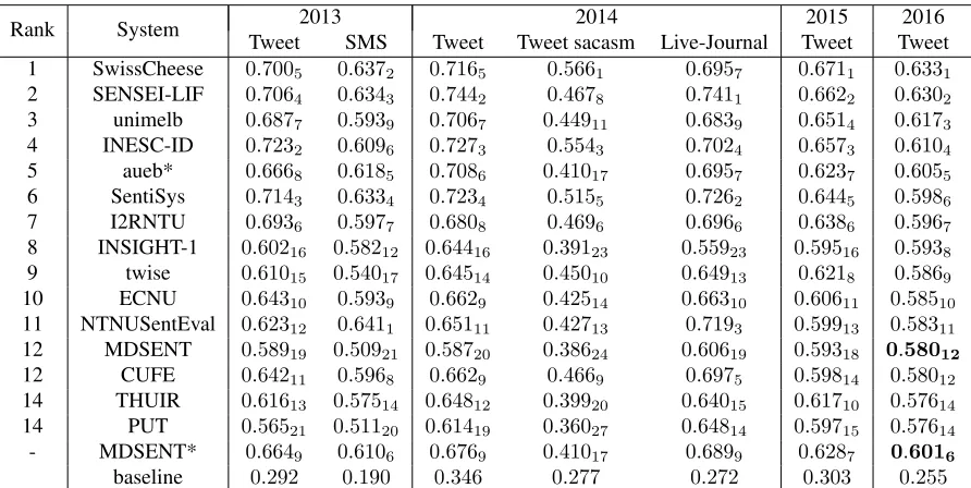
baseline 0.292 0.190 0.346 0.277 0.272 0.303 0.255 Table 3: Evaluation Results of the top 15 systems with ranks provided as subscripts. aueb* stands for ”aueb.twitter.sentiment”. Our model with setting 1 ranks 12th among 34 systems. We also show the evaluation results and our reported ranks of MDSENT with setting 2 among the 34 systems in MDSENT*.

Runs _wSetting 1 Setting 2

F₁P N w F₁P N

Run 1 0.66 0.582 1.00 0.603 Run 2 0.81 0.583 1.00 0.604 Run 3 0.60 0.587 0.98 0.607 Run 4 0.60 0.591 0.97 0.603 Run 5 0.60 0.592 0.95 0.601 Average 0.654 0.587 0.98 0.604 Table 4:Statistics of 5 individual runs for both settings.

We show the evaluation results of our system in Table 3, along with the top 15 systems reported. Originally we tested the system with only setting 1 and it ranks 12th among 34 systems. However, we find the system with setting 1 perform poorly on older datasets, which may due to the lack of train-ing data. Thus we then test our model with setttrain-ing 2 and report ranks generated from the same list of evaluation results reported by the 34 systems. It is apparent that our system can benefit from more training data and shows significant performance im-provement (rank 6th).

Another interesting observation is that when pro-vided with large amounts of training data, the CNN itself can perform very well, with LR assigned a very small weight during the combination

proce-dure. We further test this finding by making 5 indi-vidual runs for both settings and checking the com-bination scalar weightw and final evaluation score FP N

1 . We list corresponding results in Table 4. With

more training data,wincreased from an average of

0.654to an average of 0.98, which is very close to

1, while the performance improved from an aver-age of0.587to an average of0.604. This suggests

the possibility to use only deep learning techniques along with embeddings to achieve similar or even better performance than traditional systems that re-quire a lot of human engineered features and knowl-edge bases.

Our future work includes finer-design of the CNN, e.g., performing two stages of classification: first for subjectivity detection and then for polar-ity classification. We will also seek the possibilpolar-ity of conducting unsupervised learning with the CNN, which allows us to make use of the large amount of tweets on the Internet. With such increased amount of training data, our system may further improve its performance.

References

Natural language processing (almost) from scratch.

The Journal of Machine Learning Research, 12:2493– 2537.

Kevin Gimpel, Nathan Schneider, Brendan O’Connor, Dipanjan Das, Daniel Mills, Jacob Eisenstein, Michael Heilman, Dani Yogatama, Jeffrey Flanigan, and Noah A Smith. 2011. Part-of-speech tagging for twit-ter: Annotation, features, and experiments. In Pro-ceedings of the 49th Annual Meeting of the Associa-tion for ComputaAssocia-tional Linguistics: Human Language Technologies: short papers-Volume 2, pages 42–47. Association for Computational Linguistics.

Geoffrey E Hinton, Nitish Srivastava, Alex Krizhevsky, Ilya Sutskever, and Ruslan R Salakhutdinov. 2012. Improving neural networks by preventing co-adaptation of feature detectors. arXiv preprint arXiv:1207.0580.

Minqing Hu and Bing Liu. 2004. Mining and summa-rizing customer reviews. InProceedings of the tenth ACM SIGKDD international conference on Knowl-edge discovery and data mining, pages 168–177. ACM.

Yoon Kim. 2014. Convolutional neural networks for sen-tence classification.arXiv preprint arXiv:1408.5882. Tomas Mikolov, Kai Chen, Greg Corrado, and Jeffrey

Dean. 2013a. Efficient estimation of word representa-tions in vector space. arXiv preprint arXiv:1301.3781. Tomas Mikolov, Ilya Sutskever, Kai Chen, Greg S Cor-rado, and Jeff Dean. 2013b. Distributed representa-tions of words and phrases and their compositionality. InAdvances in neural information processing systems, pages 3111–3119.

Saif M Mohammad and Peter D Turney. 2010. Emo-tions evoked by common words and phrases: Using mechanical turk to create an emotion lexicon. In Pro-ceedings of the NAACL HLT 2010 workshop on com-putational approaches to analysis and generation of emotion in text, pages 26–34. Association for Compu-tational Linguistics.

Saif M Mohammad, Svetlana Kiritchenko, and Xiaodan Zhu. 2013. Nrc-canada: Building the state-of-the-art in sentiment analysis of tweets. arXiv preprint arXiv:1308.6242.

Preslav Nakov, Alan Ritter, Sara Rosenthal, Fabrizio Se-bastiani, and Veselin Stoyanov. Evaluation measures for the semeval-2016 task 4 ’sentiment analysis in twit-ter’(draft: Version 1.1).

Finn ˚Arup Nielsen. 2011. A new anew: Evaluation of a word list for sentiment analysis in microblogs. arXiv preprint arXiv:1103.2903.

Richard Socher, Eric H Huang, Jeffrey Pennin, Christo-pher D Manning, and Andrew Y Ng. 2011. Dynamic

pooling and unfolding recursive autoencoders for para-phrase detection. InAdvances in Neural Information Processing Systems, pages 801–809.

Theresa Wilson, Janyce Wiebe, and Paul Hoffmann. 2005. Recognizing contextual polarity in phrase-level sentiment analysis. InProceedings of the conference on human language technology and empirical methods in natural language processing, pages 347–354. Asso-ciation for Computational Linguistics.