A constrained graph algebra for semantic parsing with AMRs

A constrained graph algebra for semantic parsing with AMRs

Jonas Groschwitz∗† Meaghan Fowlie∗ Mark Johnson† Alexander Koller∗ ∗

Saarland University, Saarbr¨ucken, Germany †Macquarie University, Sydney, Australia

jonasg|mfowlie|[email protected] [email protected]

Abstract

When learning grammars that map from sentences to abstract meaning representations (AMRs), one faces the challenge that an AMR can be described in a huge number of different ways using traditional graph algebras. We introduce a new algebra for building graphs from smaller parts, using linguistically motivated operations for combining a head with a complement or a modifier. Using this algebra, we can reduce the number of analyses per AMR graph dramatically; at the same time, we show that challenging linguistic constructions can still be handled correctly.

1

Introduction

Semantic parsers are systems which map natural-language expressions to formal semantic representa-tions, in a way that is learned from data. Much research on semantic parsing has focused on mapping sentences to Abstract Meaning Representations (AMRs), graphs which represent the predicate-argument structure of the sentences. Such work builds upon the AMRBank (Banarescu et al.,2013), a corpus in which each sentence has been manually annotated with an AMR.

The training instances in the AMRBank are annotated only with the AMRs themselves, not with the structure of a compositional derivation of the AMR. This poses a challenge for semantic parsing, especially for approaches which induce a grammar from the data and thus must make this compositional structure explicit in order to learn rules (Jones et al.,2012,2013;Artzi et al.,2015;Peng et al.,2015). In general, the number of ways in which an AMR graph can be built from its atomic parts, e.g. using the generic graph-combining operations of the HR algebra (Courcelle,1993), is huge (Groschwitz et al.,

2015). This makes grammar induction computationally expensive and undermines its ability to discover grammatical structures that can be shared across multiple instances. Existing approaches therefore resort to heuristics that constrain the space of possible analyses, often with limited regard to the linguistic reality of these heuristics.

We propose a novel method to generate a constrained set of derivations directly from an AMR, but without losing linguistically significant phenomena and parses. To this end we present anapply-modify (AM) graph algebra for combining graphs using operations that reflect the way linguistic predicates combine with complements and adjuncts. By equipping graphs with annotations that encode argument sharing, AM algebra derivations can model phenomena such as control, raising, and coordination straig-htforwardly. We describe a method to generate the AM algebra for an AMR in practice, and demonstrate its effectiveness: e.g. for graphs with five nodes, our method reduces the number of candidate terms from 1017_{to just21on average.}

2

Related work

swallow

chew manner

snake

ARG0

prey

ARG1 ARG0

ARG1

-polarity

poss

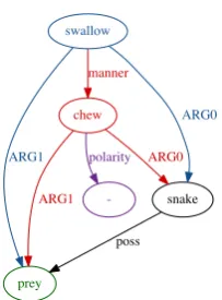
Figure 1: AMR of The snake swallows its prey without chewing.

This paper is concerned with finding the hidden compositional structure of AMRs, the semantic representations annotated in the AMRBank (Banarescu et al.,2013). AMRs are directed, acyclic, rooted graphs with node labels in-dicating semantic concepts and edge labels inin-dicating semantic roles, such as argumentsARG0,ARG1, . . . and modifiers, such as manner and time.

An example is shown in Fig.1.1 Here, snake is anARG0of both chew

andswallow, andpreyis anARG1ofswallow. Nodes can fill argument posi-tions of multiple predicate nodes, not just because of grammatical phenomena such as control, but also because of coreference (itsprey), or because they are pragmatically implied arguments (edge fromchew toprey). An AMR’s root represents a “focus” in the graph; the root is often the main predicate of the sentence. In Fig. 1, the root is theswallownode. AMRs are “abstract” be-cause they gloss over certain details of the syntactic realization. For example,

destruction of Rome andRome was destroyed have the same AMR; among others, tense and determiners are dropped.

The availability of the AMRBank has spawned much research on semantic

parsing into AMR representations. The work in this paper is most obviously connected to research that models the compositional mapping from strings to AMRs with grammars – using either synchronous grammars (Jones et al.,2012;Peng et al.,2015) or CCG (Artzi et al.,2015;Misra and Artzi,2016). Not all AMR parsers learn explicit grammars (Flanigan et al.,2014;Peng et al.,2017). However, we believe that these, too, may benefit from access to the compositional structure of the AMRs, which the algebra we present makes easier to compute.

The operations our algebra uses to combine semantic representations are closely related to those of the “semantic algebra” of Copestake et al.(2001), which was intended to reflect universal semantic combination operations for large-scale handwritten HPSG grammars. More distantly, the ability of our semantic representations to select the type of its arguments echoes the use of types in Montague Grammar and in CCG (Steedman,2001), applied to graphs.

3

Algebras for constructing graphs

We start by reviewing the HR algebra and discussing some of its shortcomings in the context of grammar induction. Then we introduce the apply-modify graph algebra, which tackles these shortcomings in a linguistically adequate way.

Notation:For a given (partial) functionf :A_→B, we write_D(f)_⊆Afor the set of values on whichf is defined andI(f)_⊆Bfor its image. When convenient, we read functions as sets of input-output pairs, so that e.g.∅denotes the partial function that is undefined everywhere. Iff, gare (partial) functions, we writef_◦gfor the functionhsuch thath(a) =f(g(a))for alla. Iff is injective, we writef−1_{for its} inverse (partial) function. We writef for the total function such thatf(a) =f(a)iff(a)is defined and f(a) = aotherwise. Finally, for an input valuex ∈ D(f), we writef \xfor the function that is equal tof except that it is undefined onx.

AΣ-algebraA= hA,(f)F∈Σiis a structure in which terms over asignatureΣcan be evaluated as

elements from the algebra’sdomain_A. Here,Σis aranked signature; that is, a set of symbolsF ∈ Σ,

each of which is equipped with arank_∈N. Symbols of rank 0 are calledconstants. For eachF ∈Σof rankk, the algebra defines a functionf :_Ak _{→ A; in particular, constants are interpreted as elements}

ofA. The functions may be partial; thenAis called apartialalgebra. We define thetermsoverΣ,TΣ, recursively: all constants are terms, and ifF ∈Σhas ranknandt1, . . . , tn ∈TΣ, thenF(t1, . . . , tn)is

1

APPO

Gtv[love] Gn[rose] (a) AM term

fO

||

Gtv[love] renrt7→O

Gn[rose] (b) HR term

����

��

�

����

�

����

(c)Gtv[love]

����

��

����

�

(d) renrt7→O

inGn[rose]

���� ��

� ����

���� � ����

(e) Merge c and d

����

��

�

����

���� ����

(f) ForgetOsource

Figure 2: HR algebra derivation ofloves a rose.

also a term. Such a termevaluatesrecursively to the valueJtK =f(Jt1K, . . . ,JtnK) ∈ A. Approaching

graphs algebraically allows us to examine the compositionality of graphs – how graphs can be built from smaller graphs. For example, the terms in Figures2aand2bboth describe the combining of the graphs in Figures2cand2dto form the graph in Fig.2f. We describe the operations used in these terms in the following subsections.

Convention: To increase readability and since in this paper we focus on the functions and rarely refer to a symbol itself, we will denote a function corresponding to a symbol with the symbol itself. I.e. we will use the same notation for both symbol and associated function, not making the distinction between

Fandfas in the definition above. But as a general principle in this paper, this common notation always refers to the function in text and definitions, and to the symbol in terms such as in Figures2aand2b.

3.1 S-graphs and the HR algebra love

rt

prince ARG0

rose ARG1

(a) AMR

fX

||

||

renrt7→X

Nrose

||

EARG1 renX7→rt

frt

||

ren_X7→rt,rt7→X

EARG0

Nprince Nlove

(b) HR term

Figure 3: AMR generated by linguistically bizarre HR term A standard algebra for the theoretical literature for describing graphs

is the HR algebraof Courcelle (1993). It is very closely related to hyperedge replacement grammars (Drewes et al., 1997), which have been used extensively for grammars of AMR languages (Chiang et al.,

2013;Peng et al.,2015), andKoller (2015) showed explicitly how to do compositional semantic construction using the HR algebra.

The objects of the HR algebra ares-graphsG= (g, S), consisting of a graphg(here, directed and with node and edge labels) and a par-tial functionS : _S V, which mapssourcesfrom a fixed finite set S of source names to nodes ofg. Sources thus serve as external, inter-pretable names for some of the nodes. If we haveS(a) = v, then we callvana-sourceofG. An example of an s-graph with a root-source (rt) and a subject-source (S) is shown in Fig.2f. Sources are marked in diagrams asrednode labels.

The HR-algebra serves as a compositional algebra for graphs be-cause it includes an operationmergewhich connects two graphs at the nodes that share source names. The algebra evaluates terms from a signature which, in addition to constants for s-graphs, contains three further types of function symbols. Themergeoperation||, of rank two, combines two s-graphsG1 andG2 into a new s-graphG0that contains all the nodes and edges ofG1andG2. IfG1has ana-sourceuandG2 has ana-sourcev, for some source namea, thenuandvwill be map-ped to the same node inG0, taking with it all the edges into and out ofu andv. We will usually write_||in infix notation. Therenameoperation ren{a17→b1,...,an7→bn}, of rank one, renames the sources of an s-graph; if

the nodeuwas anai-source before the rename, it becomes abi-source.

Finally, theforgetoperationfa, of rank 1, removes the entry for source

afromS, i.e. the resulting s-graph no longer has ana-source.

Fig.4with “love” and “rose”, respectively. The termrenamesthe rt-source ofGn[rose]to anO-source (Fig. 2d). Thus when the result ismerged withGtv[love], the “rose” label is inserted into the object position of the verb (Fig.2e). Finally, weforgettheO-source, yielding the s-graph in Fig.2f.

The operations of the HR algebra are rather fine-grained, and can be combined flexibly. This is an advantage when developing grammars using the HR algebra by hand (Koller,2015), but makes the automatic induction of grammars from the AMRBank expensive and error-prone. Groschwitz et al.

(2015) show that with more than three sources, the problem becomes quite extreme, and that with such few sources available, one must use constants of only one or two nodes. Following the experimental setup ofGroschwitz et al.(2015),Nrose,Nprince andNlovein Figure3bevaluate to labelled nodes with a

rt-source, andEARG0andEARG1evaluate to single edges with a rt-source at their source and anX-source at their target. Using these constants and just the two sources rt andX, there are already 3584 terms over the HR algebra which evaluate to the (quite small) s-graph in Fig.3a.

This set of terms is riddled with spurious ambiguity and linguistically bizarre analyses, such as the term shown in Fig.3b. Two strange aspects of this example are: one,princebecomes an X-source by first switching X and rt and then switching them back; this step is unnecessary and inconsistent with the corresponding process for rose here. Two, prince and rose are combined with empty argument connectors beforelovefinally is inserted as the predicate, despite these roles being originally defined in

love’s semantic frame.

Not only does this make graph parsing computationally expensive (Chiang et al.,2013;Groschwitz et al., 2015), it also makes grammar induction difficult. For example, Bayesian algorithms sample random terms from the AMRBank and attempt to discover grammatical structures that are shared across different training instances. When the number of possible terms is huge, the chance that no two rules share any grammatical structure increases, undermining the grammar induction process. Existing sys-tems therefore apply heuristics to constrain the space of allowable HR terms. However, these heuristics are typically ad-hoc, and not motivated on linguistic grounds. Thus there is a risk that the linguistically correct compositional derivation of an AMR is accidentally excluded.

3.2 The apply-modify graph algebra

Figure 4: Lexicon. ** can be replaced by a label of the right category. Examples:Gtv: love,Giv: sleep;Gunacc:

relax;Gmod: red;Gn: prince,rose,sheep,pilot;Gscv: want; Gocv: persuade;Gc-[s]: and (seeking operands of type

[S]). rt stands forroot,Sforsubject,Oforobject, and mod formodifier.

Upon closer reflection, the structure of the HR term in Fig.2bis not arbitrary. Many semantic theories assume that two key operations in combining semantic representations compositionally areapplication

Apps

Appo s

Gscv[want] s,o[s]

Gunacc[relax] s Gn[sheep]

(a) Term

want rt

relax ARG1

sheep ARG0

ARG1

(b) AMR

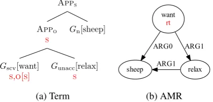
Figure 5: Subject controlThe sheep wants to relax

APPO2

S,O

Gocv[persuade] S,O, O2[S][S7→O]

Giv[go] S

(a) Term

persuade

rt

S

ARG0

O

ARG1

go ARG2

ARG0

(b) AMR

Figure 6: Object control:persuade to go

3.2.1 Application

We first define theapplyoperation APPα, whereαis a source name. In the simple case of Fig.2a, APPO

renames the rt-source of its second argumentG2toO, merges the result with the first argumentG1, and then forgetsO – just as in the HR term in Fig.2b, but with a single algebra operation.

In this simple case,G2 was complete; its only source was rt. However, in certain cases, we want to combine a predicate with an argument that is itself still looking for arguments. Take the graph in Fig.5b

for example, corresponding to the sentence “the sheep wants to relax”, where the sheep is both the wanter and the relaxer. For the subject control verbwant, we use the lexicon entry Gscv[want]of Fig.4. Its

O source is annotated with the argument type S (written O[S]). This means thatGscv[want]requires its object argument to contain an S-source; during application this node is merged with theS-source of Gscv[want]itself. This yields a graph with an (undirected) cycle, that is, a graph that is not a tree.

We also allow annotations forrenamingsources, in order to model phenomena such as object control verbs, as in “the prince persuaded the sheep to sleep” (see Fig.6a-b). Here,sheepis both the subject of

sleepand the object ofpersuade. We can handle this with the graph forGocv[persuade]in Fig.4, that features anO2-source which is annotated asO2[S][S7→O]. ThisO2-source must be filled by a graphG2 that still has anS-source, which is renamed to anO-source during application, and thus merged with the

O-source of persuade. This yields the structure shown in Fig.6b. To capture these intuitions formally, we present the following definitions.

Definition 3.1 (Graph types (TY)). Agraph type is a pair τ = (T, R) of a function T : S _→ TY, where S _{⊆ S} is a set of source names, that assigns a graph type to each source, and a function R : S → {r :S S |rpartial, injective} that annotates each source with a renaming function. R may only rename sourcesT requires , i.e. we demand_∀T(α) =_hT0, R0_i,_D(R(α)) _{⊆ D}(T0). We say thatSis thedomainofτ. Intuitively, the graph typeτ provides annotations for all source names inS.

Definition 3.2 (Annotated s-graph (as-graph)). Anannotated s-graph (as-graph)is a pair_G=_hG, τ_i of an s-graphG = (g, S)that contains a “root” source (i.e. rt ∈ D(S)) and agraph typeτ ∈TY with domainS_{\ {}rt_}. We write_ASfor the set of all as-graphs.

Our notation, as seen in the above examples, follows the patternα[T(α)][R(α)]for a sourceαand its annotation, but we simplify it and drop empty types and functions. For example, the notation O in Gtv[love]indicates thatT(O) = (∅,∅)andR(O) = ∅. The notationO[S] inGscv[want]indicates that

T(O) = ({S 7→ (∅,∅)},{S 7→ ∅}) and R(O) = ∅. That is, we require the argument to have an S -source that itself is not further annotated, and we do not rename it. Finally, the notationO2[S][S7→O] in

Gocv[persuade]indicates that similarlyT(O2) = ({S7→(∅,∅)},{S 7→ ∅}), but nowR(O2) ={S7→ O}, signalling the rename.

Definition 3.3 (Apply operation (APP)). LetG1 = ((g1, S1),(T1, R1)),G2 = ((g2, S2),(T2, R2))be as-graphs. Then we let APPα(G1,G2) = ((g0, S0),(T0, R0))such that

(g0, S0) =fα((g1, S1)||ren{rt7→α}(renR1(α)((g2, S2)))) T0 = (T1\ {α})∪(T2◦R1(α)−1)

R0 = (R1\ {α})∪(R2◦R1(α)−1)

1. G1actually has anα-source to fill, i.e.α_{∈ D}(T1),

2. G2has the typeαis looking for, i.e.T1(α) = (T2, R2), and 3. T0, R0are well-defined (partial) functions;

otherwise APPα(G1,G2)is undefined.

The interpretation is just as discussed at the start of Section 3.2 above: we apply all renamings required byR1 to(g2, S2), we rename the root toα, we merge the graphs, and then we forget α. The type of the output graph,(T0_{, R}0_{), is defined such that the source we just filled,α, is removed, and the} renaming function ofG1atαis applied to the domains ofT2andR2, so that any requirementsG2had on its arguments are properly carried over into the new renamed graph. Conditions1and2ensure that the operation matches the intuition behind the source annotations. Condition3guarantees that there are no conflicts in the remaining source annotations of the two graphs. Note that sinceT1(α) equals the type (T2, R2)if Condition2holds, the type(T1, R1)can then alone guarantee Condition3. Observe that the term in Fig. 2agenerates the as-graph in Fig.2f; in both Figures5 and6, the term in (a) generates the graph in (b).

3.2.2 Modification

MODMOD

Gn[rose] Gmod[red] MOD

(a) AM term

||

Gn[rose] renMOD7→rt

frt

Gmod[red] (b) HR term

rose

rt

red mod

(c) AMR

Figure 7: Modification:a red rose

We further define a modify operation MODα,

which models modification of its first argument G1 by its second argument G2. An example of using MODMOD to construct an as-graph for “red

rose” is shown in Fig.7, where the modify ope-ration captures the HR term in Fig. 7b: We for-get the rt-source of the as-graph Gmod[red]; re-name itsMOD-source to rt; and then merge it with

Gn[rose]. That is, we shift the rt-source of the modiferG2to the unlabelledMOD-source and attach it at the root ofG1. This yields the AMR in Fig.7c. Unlike in the apply case, we can repeat this modification operation as many times as we like: no sources ofG1are forgotten.

Definition 3.4 (Modify operation (MOD)). In general, we define the modify operationfor a sourceα as follows. Again, let G1 = ((g1, S1),(T1, R1)),G2 = ((g2, S2),(T2, R2))be as-graphs. Then we let

MODα(G1,G2) = ((g0, S0),(T1, R1))such that

(g0, S0) = (g1, S1)||ren{α7→rt}(frt((g2, S2))) if and only if

1. α_{∈ D}(τ2), i.e.G2has anαsource,

2. T2(α) = (∅,∅), i.e. G2does not have complex expectations atα, and

3. T2\α ⊆T1andR2\α⊆R1, i.e. any remaining sources and annotations inG2are already inG1;

otherwise it is undefined.

Again, the s-graph evaluation and Condition1are straightforward. Modification is more restricted then application, and we demand that the modifier does not change the modifiee’s type (Condition 3). We do however allow additional sources in G2 to merge with existing ones ofG1. For example, when

chewwould modifyswallowto create the graph in Fig.1(“without chewing”), their subject and object would merge. Condition2avoids using e.g. the control structure ofGscv[want]for modification.

We conclude this section by defining theapply-modify graph algebra (AM algebra)as an algebra whose domain is the set of all as-graphs. In addition to constants (which evaluate to as-graphs), the AM algebra’s signature contains the symbols APPα (of rank 2) and MODα(of rank 2). The associated

4

Linguistic Discussion

The AM algebra restricts the derivations for a given AMR. The danger, then, is that we could lose all derivations for an AMR, making it unparseable, or that the terms we are left with are not linguistically reasonable. In this section, we show we find reasonable terms for a range of challenging examples. A quantitative analysis of the amount of graphs in the AMRBank for which we can find a decomposition is provided in Section6.

Apps

Appo

s

Gscv[want]

s,o[s]

Appop2 s

Appop1 op2[s]

Gc−[s][and]

op1[s] op1[s]

Giv[sleep]

s

Gunacc[relax]

s Gn[sheep]

(a) Term

���

��

����� ���

����� ���

�

���� ����

(b) sleep and relax

want

rt and

ARG1

sheep ARG0 sleep

op1

relax op2

ARG0 ARG1

(c) The sheep wants to sleep and relax.

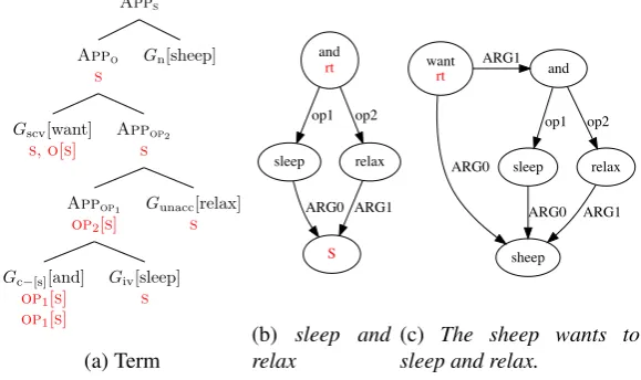
Figure 8: Conjoining intransitive verbs We have already seen how to

derive simple argument application, modification, and control constructi-ons. APP is designed explicitly to

parallel for example beta-reduction in lambda calculus, and syntactic operations such as forward and backward application in categorial grammars or endocentric context-free rules. The two arguments of the function combine in such a way that one is in a sense inserted into the ot-her, and the operation is only per-mitted if the types are correct. In an AM-algebra, APPα is only allowed

if the first argument’s type includes the sourceα, and the second argument’s type isT1(α), and the result is a graph in which the first argument keeps its original root, and the second graph is inside the first.MOD

is designed to parallel for example modification of phrases by phrases in a context-free grammar, or mo-dification as X/X categories in categorial grammars: the type of the modifier is a subset of the modified graph, so that modification has no effect on the type of the modified graph, and the modification happens at the root. Modification can also derive control insecondary predicatesthat modify the verb phrase and link an argument to an argument of the verb. For example, to derive(1), the graph forwithout dreaming

modifiesGiv[sleep]while both have an openS-source.

(1) The princeislept [without [ idreaming]]

4.1 Coordination

Coordination is a source of re-entrancies in AMRs. For example, when two verb phrases are conjoined, as in(2-a), their subjects must co-refer. Objects can also co-refer in English, as in(2-b). Control verbs, which already have re-entrencies of their own, can be conjoined, as in(2-c). Even subject- and object-control verbs can be conjoined if the object object-control verb is in the passive(2-d).

(2) a. The princei isang and idanced

b. The princei igrew jand iloved ja rosej c. The sheepi iwanted and ineeded ito relax

d. The princejwanted jto gov, or jwas persuaded jto v. e. The rosei[asked j v] and i[persuaded the Princejto stayv].

Coordination is generally observed to be between like things; for us this mean the arguments have the same type. For example, in Fig.8, we choose anandthat chooses arguments that are missing their subject – it has annotated sourcesOPi[S]. WhenGiv[sleep]andGunacc[relax]merge, so do their subjects. In this way, the graph forsleep and relaxcan be selected by a control verb,Gscv[want], merging its subject with theirs. Similarly, for example(2-e),askandpersuadeare conjoined by a conjunctionandwhich is look-ing for two object-control verbs; that is,andhas type{OP1[S,O,O2[S][S7→O]],OP2[S,O,O2[S][S7→O]]}.

arguments – we do this in our implementation in Section5.

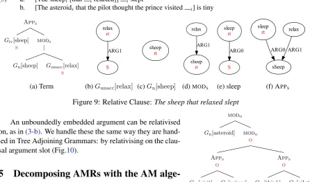
4.2 Relative Clauses

Relative clauses are unusual in that one of the arguments of a modifier is the very thing it is modifying. For example, in(3-a), the relative clausethat relaxedhassheepas the subject ofrelax, andthat relaxed

modifiessheep. To capture this, we includeMODSandMODO in our repertoire. For a subject relative we

make the subject into the root and use it to modifysheep, as in Figure9.

(3) a. [The sheepi[that irelaxed]] islept

b. [The asteroidithat the pilot thought the prince visited i] is tiny

Apps

Giv[sleep] s

mods |

Gn[sheep] Gunacc[relax] s (a) Term relax rt S ARG1

(b)Gunacc[relax]

sheep rt

(c)Gn[sheep]

relax

sheep rt

ARG1

(d)MODS

sleep rt S ARG0 (e) sleep sheep sleep rt ARG0 relax ARG1

(f) APPS

Figure 9: Relative Clause:The sheep that relaxed slept

modo

Gn[asteroid] modo o

Apps o

Gtv[visit] s,o

Gn[prince]

Apps o

Gtv[think] s,o

Gn[pilot]

Figure 10: the asteroid the pilot thinks the prince visited

An unboundedly embedded argument can be relativised on, as in(3-b). We handle these the same way they are hand-led in Tree Adjoining Grammars: by relativising on the clau-sal argument slot (Fig.10).

5

Decomposing AMRs with the AM

alge-bra

At this point, we have defined the AM algebra – as a more constrained algebra of graphs than the HR algebra – and shown the adequacy of the apply and modify operations for

a number of nontrivial linguistic examples. We will now show how to enumerate AM terms that evaluate to a given graph, e.g. an AMR in the AMRBank. As indicated above, this is a crucial ingredient for grammar induction.

The first step in decomposing a graph G in this way is to select the constants for as-graphs that we will use in the AM algebra – i.e., “atomic” as-graphs such as those in Fig. 4. During grammar induction, we have no grammar or lexicon to draw from, so we will use heuristic methods to extract constants from G. Throughout, we assume thatGis an AMR, and we will use a fixed set of sources S =_{rt,S,O,O2, . . . ,O9,MOD,POSS,DOMAIN} ∪ {OPx|opxedge label occurs in the corpus}.

5.1 Constants and their types lovert

prince ARG0 rose ARG1 (a)G prince rt

(b)sprince rose

rt

(c)srose

love rt S ARG0 O ARG1

(d)slove-active

love rt S ARG1 O ARG0

(e)slove-passive

Figure 11: (a) An AMRG; (b)-(e) the constants we obtain We start by cutting Gup into the

subgraphs that will serve as graph backbones of the constants. We do this by splitting G into blobs. A blob consists of a main labeled node and itsblob edges, which are the node’s outgoing edges with an

defined in this way uniquely partition an AMR’s edge set. An example of an AMR’s blobs is shown in Fig.1, where the blobs are distinguished by colour. For example, thechewblob is the red subgraph, in-cluding unlabelled nodes where ever a red edge touches a non-red node. These unlabelled endpoints are itsblob-targets. We will construct a set of constants for each blob, such that the value of each constant is an as-graph whose graph component is the blob. The main node of the blob will be the rt-source. It remains to assign source names to the blob-targets and annotate them with types and renaming functions. The different choices of annotated source names constitute the different constants for this blob.

5.1.1 Source names

We heuristically assign (syntactic) source names from_Sto the blob-target nodes based on the edge label of their adjacent edge in the blob. Let vbe a node. Canonically, we use the following edge-to-source mapping E2S to determine sources forv’s blob-targets: For most nodesv, E2S mapsARG0toS;ARG1

toO and otherARGx toOx;possandparttoPOSS;sntx,opx anddomainto themselves; and all other

edges toMOD. Exceptionally, ifvhas a node label that is a conjunction2and at least two outgoingARGx

edges, we mapARGxtoOPxinstead. E2S determines the canonicaltarget-to-source mappingbv, which

assigns a source to each blob-targetu: if the edge betweenvanduhas labele,bv(u) = E2S(e). When

decomposing the graph in Figure11a, looking at thelovenode asv, this gives us the constant in Figure

11d.

A given blob may generate more than one constant, each with different sources on different nodes; accordingly, for each node v in G, we collect a set B(v) of such target-to-source mappings. B(v) contains the canonical mapping bv, and we generate further target-to-source mappings by applying a

fixed set of lexical rules tobv. Thepassiverule switchesS with any O, andobject promotion mapsOi

toOi−1 (letO0=O). We allow all results of such mappings with at most one use ofpassivethat have no duplicate source names. For example, the constant in Figure11eis a result of the passive rule. For each mapping inB(v), we create a constant with the respective sources and trivial types.

5.1.2 Annotations wantrt

S ARG0

O ARG1

(a) trivial types

want rt

S ARG0

O[S] ARG1

(b) non-trivial types

Figure 12: Possible source assign-ments for the want constant for the graph in Figure5b.

We can also use these target-to-source mappings to extract con-stants that have sources with non-trivial argument types and re-naming functions. Consider the subject-control AMR in Fig.5b in section 3.2.1 above. So far, we obtain the constant in Fig.12a, but we also want to generate the constantGscv[want] in Fig.12b; i.e. determine theSentry inT(O). Writingvwant,

vsheep, and vrelax for the want, sheep, and relax nodes of the

graph in5b, note that it is theARG1edge fromvrelaxtovsheep

that signals the control structure. That is,vwanthas a blob-target

vrelax, and the two share a common blob-targetvsheep. For such a triangle structure, we consider any

target-to-source mappings mw ∈ B(vwant) and mr ∈ B(vrelax). We then add a constant for vwant

which as before uses the source names ofmw, but now the annotation ofmw(vrelax)has an entry for

mr(vsheep), anticipating the open source coming from thevrelax constant. We add a rename annotation

[mr(vsheep)7→mw(vsheep)] if necessary. That is, we set up the annotation in thevwantconstant such that

when we apply it to avrelaxconstant that has sources according tomr, we obtain the structure we found

in the graph. Take for example mw = {vrelax 7→ O, vsheep 7→ S} andmr = {vsheep 7→ S}.3 In this case, mw(vsheep) = mr(vsheep) = S, therefore no rename is necessary and we obtain the constant of

Figure12b. If we choosemr = {vsheep 7→ O} instead, we obtain a constant for thevwant blob where

theOsource is annotatedO[O][O7→S]. In this graph, this is not particularly meaningful from a linguistic perspective, but in other graphs this principle allows us to generate e.g. the object control structure of

2

According to the AMR documentation, these areand,or,contrast-01,eitherandneither. 3

Gocv[persuade]. To ensure that we recover the correct constant, we simply add constants for all choices

ofmw ∈B(vwant)andmr∈B(vrelax).

Let us now find the constants for the and node in Fig. 8b. Our algorithm restricts constants to coordination of like types. In the intended AM term, shown in Fig.8a, we first coordinaterelax and

sleepbefore we apply the result to the common argumentsheep. To generate the constant forand, we consider mapsms ∈ B(vsleep)andmr ∈B(vrelax), wherevsleepandvrelaxare the nodes labelledsleep

andrelaxrespectively. Thesheepnodevsheepis a blob-target of bothvsleepandvrelax. If additionally the

target-to-source maps agree, e.g.ms(vsheep) =mr(vsheep) =S, we add a new constant for theandblob

where bothT(OP1) andT(OP2)have anS entry. This yieldsGc−[s][and]as depicted in Fig.4. For the case where ms(vsheep) = S butmr(vsheep) = O, we do not create a new constant. Again, we take all combinations of choices formsandmrinto account. We never rename for coordination.

Similar patterns allow us to find possible raised subjects for raising constructions, and to handle coordination of control verbs. Using these patterns recursively, we can handle nested control, coordi-nation and raising constructions. For example in Fig.8c, finding thesheepnode as a common target in coordination allows us to generateGscv[want]analogously to Fig.5b.

In sum, we obtain types and renaming functions that cover a variety of phenomena, in particular the ones described in Section4.

5.2 Coreference

In the AMRBank annotations, the same node can become the argument of multiple predicates in two very different ways: because the grammar specifies it (as with control, (4-b)), and through accidental coreference(4-a).

(4) a. Maryithinks shei/j’s a genius b. Maryiwants ito be a genius

Because accidental coreference is not a compositional phenomenon, we add an extra mechanism for handling it. We followKoller (2015) in introducing special sourcesCOREF1,COREF2,. . . ,COREFnfor some maximaln _∈N. We add variants of the previously found constants with aCOREF source at their

root. We further add constants consisting of a single unlabelled node, which is both a rt-source and a

COREF-source. TheCOREF sources are never annotated and are ignored in the types. They are never forgotten, and each can therefore be used only on one node in the derivation. Two COREFsources with

the same index will be automatically merged together during the usual APPandMOD operations, due to the semantics of the underlying merge operation of the HR algebra.

COREF sources increase runtimes and the number of possible terms per graph significantly (see

Section6), and thus we limit the number ofCOREFsources to zero to two in practice.

5.3 Obtaining the set of terms

We can compactly represent the set of all AM terms that evaluate to a given AMR Gin a decomposi-tion automaton (Koller and Kuhlmann,2011), a chart-like data structure in which shared subterms are represented only once. We can enumerate the terms from this automaton.

To enumerate all rules of the decomposition automaton, we explore it bottom-up, with Algorithm1. We first find all constants forGin Line2, as described in Section5.1, and then repeatedly apply APP

and MOD operations (Lines3 onward; the setOcontains all relevant APP and MOD operations). The

constants and the successful operation applications are stored as rules in the automaton.

To ensure that the resulting terms evaluate to the input graphG, we use subgraphs ofGas states – like one uses spans in string parsing. This is paired with additional constraints, for example in APPα(s, s0),

Algorithm 1Agenda-chart-algorithm

1: init chart, agenda empty

2: add constants to agenda

3: whileagenda not emptydo

4: pull subgraphsfrom agenda

5: foroperationo_{∈ O}do

6: forsubgraphs0_{in chartdo}

7: ifo(s, s0_)allowedthen

8: addo(s, s0_{)to agenda}

9: end if

10: ifo(s0_{, s)allowedthen}

11: addo(s0_{, s)to agenda}

12: end if

13: end for

14: end for

15: addsto chart

16: end while Let us decompose the graphGin Figure11aas an example.

Let us call the nodes labelled “love”, “prince”, and “rose”vlove,

vprince andvrose respectively. In Line2, we add the subgraphs

of Fig. 11(b-e) to the agenda. Say we first pullsrose from the

agenda – since the chart is empty at this point, no operation is applicable. Say we pull slove-active next, and try to combine it

with the items in the chart – just srose at this point. If we try

to apply APPS, we realize that this tries to fill the node vprince

ofslove-active, but the root of srose is vrose. Thus, the operation

fails. (Trying APPS with srose as the left andslove-active as the

right child fails immediately sincesrosehas noS-source).MODS

fails similarly. However, APPO succeeds – both theO-source in

slove-activeand the rt-source insroseare atvrose– and produces the

graph in Fig. 2f. MODO fails, since it would involve forgetting

rt atvlove, and the root of the full graph must be preserved. We

therefore add the result of APPOto the agenda and move on.

To explore the possibilities for combining as-graphs

effi-ciently, we do not iterate over all graphs in Line6, but for each operation use an indexing structure based on source nodes and types.

Note that the operations in the automaton are restricted by the AM algebra’s type system. Therefore, selecting the correct constants as in Section5.1 is critical to obtaining the desired derivations. We do obtain all the terms in the examples in this paper in practice.

6

Evaluation

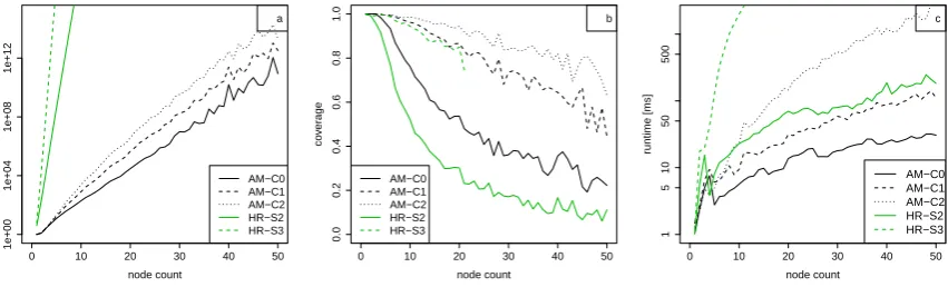
We conclude by analyzing whether the AM algebra achieves our goal of reducing the number of possible terms for a given AMR, compared to the HR algebra. Both algorithms are implemented and available in the Alto framework4. For the HR algebra, we use the setup ofGroschwitz et al.(2015): Constants consist of single labeled nodes and single edges, and they are combined using the operations of the HR algebra. We use an HR algebra with two source names S2) and one with three source names (HR-S3); this has an impact on the set of graphs that can be analyzed and on the runtime complexity. For the AM algebra, we use the method of Section5with different numbers of allowed COREF sources (AM-C0, AM-C1, AM-C2 for 0, 1, 2 COREF sources respectively). We use all graphs of the LDC2016E25 training corpus with up to 50 nodes, for a total of 35685 graphs.

0 10 20 30 40 50

1e+00 1e+04 1e+08 1e+12 node count n

umber of ter

ms AM−C0 AM−C1 AM−C2 HR−S2 HR−S3 a

0 10 20 30 40 50

0.0 0.2 0.4 0.6 0.8 1.0 node count co v er age AM−C0 AM−C1 AM−C2 HR−S2 HR−S3 b

0 10 20 30 40 50

1 5 10 50 500 node count runtime [ms] AM−C0 AM−C1 AM−C2 HR−S2 HR−S3 c

Figure 13: Number of terms per AMR (a), coverage (b) and runtimes (c).

Coverage. Consider first thecoverageof the different graph algebras, i.e. the proportion of graphs of a given size for which we find at least one term, shown in Fig.13b as a function of the graph size. As expected, coverage goes up as the number of source nodes (for HR) and COREF nodes (for AM)

increases. The coverage of AM-C0 is higher than that of HR-S2 because HR-S2 can only analyze graphs of treewidth 1, i.e. without (undirected) cycles, whereas AM-C0 can handle local re-entrancies e.g. from control constructions through the type annotations. For example, the AMRs in Fig.5b,6b can be decomposed by AM-C0 and HR-S3, but not HR-S2. The highest coverage is achieved by AM-C2.

Number of terms. We now turn to the (geometric) mean number of terms each algebra assigns to those graphs of a given size that it can analyze (Fig. 13a). We find that the AM algebras achieve a dramatic reduction in the number of terms, compared to the HR algebras: Even the high-coverage AM-C2 has much fewer terms than the very low-coverage HR-S2 (note the log-scale on the vertical axis). As an example, switching from HR-S2 to AM-C0 reduces the number of terms for the graph in Fig.3afrom 3584 to 4 (they differ in active vs passive, and order of application). For 5 nodes, the average for HR-S3 is1017_{terms, and for AM-C2 just21. This reduction has multiple reasons: we can use larger constants} in the AM algebra, and the graph-combining operations of the AM algebra are much more constrained. Further, the type system and carefully chosen set of constants restrict application and modification.

Note that just because an algebra can findsometerm for an AMR does not necessarily mean that it makes sense from a linguistic perspective (cf. Fig.3b). Conversely, by reducing the set of possible terms, there is a risk that we might throw out the linguistically correct analysis. By choosing the operations of the AM algebra to match linguistic intuitions about predicate-argument structure, we have reduced this risk. We leave a precise quantitative analysis, e.g. in the context of grammar induction, for future work.

Runtime. We finish by measuring the mean runtimes to compute the decomposition automata (Fig. 13c). Once again, we find that the AM algebra solidly outperforms the HR algebra. The runti-mes of HR-S3 are too slow to be useful in practice, whereas even the highest-coverage algebra AM-C2 decomposes even large graphs in seconds. Moreover, the runtimes for AM-C1 are faster than even for the very low-coverage HR-S2 algebra.

The previously fastest parser for graphs using hyperedge replacement grammars was the one of

Groschwitz et al. (2016), which used Interpreted Regular Tree Grammars (IRTGs) (Koller and Kuhl-mann,2011) together with the HR algebra. Because we have seen how to compute decomposition auto-mata for the AM algebra in Section5, we can do graph parsing with IRTGs over the AM algebra instead. The fact that decomposition automata for the AM algebra are smaller and faster to compute promises a further speed-up for graph parsing as well, making wide-coverage graph parsing for large graphs feasible.

7

Conclusion

In this paper, we have introduced the apply-modify (AM) algebra for graphs. The AM algebra replaces the general-purpose, low-level operations of the HR algebra by high-level operations that are specifically designed to combine semantic representations of syntactic heads with arguments and modifiers. We have demonstrated that the AM algebra dramatically reduces the number of terms for given AMR graphs, while supporting natural analyses of a number of challenging linguistic phenomena.

With this work we have laid the foundation for automatically inducing grammars that can map com-positionally between strings and AMRs while using linguistically meaningful graph-combining opera-tions. Our immediate next step will be to use the AM algebra for this purpose. On a more theoretical level, while the algebra objects differ greatly, the similarity of thesignatureof the AM algebra with that of the “semantic algebra” of Copestake et al. (2001) is striking. We will explore this connection, and investigate whether a universal signature for a semantic construction algebra can be defined.

8

Acknowledgements

References

Artzi, Y., K. Lee, and L. Zettlemoyer (2015). Broad-coverage ccg semantic parsing with amr. In Procee-dings of the 2015 Conference on Empirical Methods in Natural Language Processing, pp. 1699–1710.

Banarescu, L., C. Bonial, S. Cai, M. Georgescu, K. Griffitt, U. Hermjakob, K. Knight, P. Koehn, M. Pal-mer, and N. Schneider (2013). Abstract Meaning Representation for sembanking. InProceedings of the 7th Linguistic Annotation Workshop and Interoperability with Discourse.

Chiang, D., J. Andreas, D. Bauer, K. M. Hermann, B. Jones, and K. Knight (2013). Parsing graphs with hyperedge replacement grammars. InProceedings of the 51st Annual Meeting of the Association for Computational Linguistics.

Copestake, A., A. Lascarides, and D. Flickinger (2001). An algebra for semantic construction in constraint-based grammars. InProceedings of the 39th ACL.

Courcelle, B. (1993). Graph grammars, monadic second-order logic and the theory of graph minors. In N. Robertson and P. Seymour (Eds.),Graph Structure Theory, pp. 565—590. AMS.

Drewes, F., H.-J. Kreowski, and A. Habel (1997). Hyperedge replacement graph grammars. pp. 95–162.

Flanigan, J., S. Thomson, J. Carbonell, C. Dyer, and N. A. Smith (2014). A discriminative graph-based parser for the abstract meaning representation. In Proceedings of the 52nd Annual Meeting of the Association for Computational Linguistics (Volume 1: Long Papers), pp. 1426–1436.

Groschwitz, J., A. Koller, and M. Johnson (2016). Efficient techniques for parsing with tree automata. InProceedings of the 54th Annual Meeting of the Association for Computational Linguistics.

Groschwitz, J., A. Koller, and C. Teichmann (2015). Graph parsing with S-graph Grammars. In Pro-ceedings of the 53rd Annual Meeting of the Association for Computational Linguistics and the 7th International Joint Conference on Natural Language Processing.

Jones, B., J. Andreas, D. Bauer, K.-M. Hermann, and K. Knight (2012). Semantics-based machine translation with hyperedge replacement grammars. InProceedings of COLING.

Jones, B. K., S. Goldwater, and M. Johnson (2013). Modeling graph languages with grammars extracted via tree decompositions. InProceedings of the 11th International Conference on Finite State Methods and Natural Language Processing, pp. 54–62.

Koller, A. (2015). Semantic construction with graph grammars. InProceedings of the 11th International Conference on Computational Semantics, pp. 228–238.

Koller, A. and M. Kuhlmann (2011). A generalized view on parsing and translation. InProceedings of the 12th International Conference on Parsing Technologies.

Misra, D. K. and Y. Artzi (2016). Neural shift-reduce ccg semantic parsing. InProceedings of the 2016 Conference on Empirical Methods in Natural Language Processing.

Peng, X., L. Song, and D. Gildea (2015). A synchronous hyperedge replacement grammar based appro-ach for amr parsing. InProceedings of the 19th Conference on Computational Language Learning, pp. 32–41.

Peng, X., C. Wang, D. Gildea, and N. Xue (2017). Addressing the data sparsity issue in neural AMR parsing. InProceedings of the 15th EACL.