Question Difficulty – How to Estimate Without Norming, How to Use for Automated Grading

Question Difficulty – How to Estimate Without Norming, How to Use for

Automated Grading

Ulrike Pad´o

[email protected] Hochschule f¨ur Technik Stuttgart

Schellingstr. 24 70174 Stuttgart, Germany

Abstract

Question difficulty estimates guide test cre-ation, but are too costly for small-scale test-ing. We empirically verify that Bloom’s Taxonomy, a standard tool for difficulty es-timation during question creation, reliably predicts question difficulty observed after testing in a short-answer corpus. We also find that difficulty can be approximated by the amount of variation in student answers, which can be computed before grading. We show that question difficulty and its approximations are useful forautomated grading, allowing us to identify the optimal feature set for grading each question even in an unseen-question setting.

1 Introduction

Testing is a core component of teaching, and many tasks in NLP for education are concerned with cre-ating good questions and correctly grading the an-swers. We look at how to estimate question diffi-culty from question wording as a link between the two tasks.

From a test creation point of view, knowing ques-tion difficulty levels is imperative: Too many easy questions, and the test will be unable to distinguish between the more able test-takers, who all achieve equally good results. Too many hard questions, and only the most able test-takers will be clearly distinguishable from the (low-performing) rest.

In large-scale testing, question difficulty and other measures of question quality are established through priornorming(Downey,2010), where the questions are answered by a pool of test-takers in a dry run before definitive use with a similar de-mographic. Difficulty is then determined on the basis of the observed results using probabilistic test theory (PTT). Norming is usually not available in

automated question creation or in ad-hoc testing in small classrooms, while the need for correctly determining question difficulty of course remains. In this situation, teachers often use Bloom’s Tax-onomy (Bloom,1956), a classification of the knowl-edge dimensions and cognitive processes involved in the completion of a test task, to formulate ques-tions of appropriate difficulty. In the literature, the difficulty of multiple-choice questions has been successfully aligned with the cognitive process di-mension of the Bloom hierarchy (Tiemeier et al. (2011);Kim et al.(2012), but see alsoKibble and Johnson (2011)). In this paper, we empirically evaluate the predictive power of both Bloom di-mensions for estimating the empirically observed difficulty ofshort-answer questions, which require the test-taker to freely formulate one to three sen-tence answers. We find that the Taxonomy allows a useful approximation of question difficulty at the time of question creation. We find clear empirical evidence that theinstructional context, that is the teaching materials presented in instruction, has to be taken into account when determining difficulty using the Taxonomy.

Once test-taker answers are available, but be-fore grading makes PTT analysis possible, another predictor for question difficulty becomes available: Answer variation, the average amount of variation within the student answers for each question, is computed based only on the answer strings.

We also look at question difficulty from the point of view of improving automated short-answer grad-ing (SAG). To date, the focus of research has been on finding informative features, ranging from deep processing (Zesch et al.,2013;Hahn and Meurers, 2012) through text-based similarity (Sultan et al., 2016) to shallow, string-based approaches (Okoye et al.,2013;Jimenez et al.,2013). Pad´o(2016) has proposed to perform pre-grading model selection by tailoring feature sets to the characteristics of

different short-answer corpora. We refine this idea and show that within the same corpus, questions with different difficulty levels also profit from dif-ferent feature sets, and that the Bloom Taxonomy levels and student answer variation can be used as stand-ins for feature set prediction if difficulty estimates are not available. These results point to a new avenue of research in SAG.

The paper is structured as follows: We begin by providing some theoretical background on PTT and Bloom’s Taxonomy in Section 2. Our first set of analyses tests the reliability of the Bloom’s Taxonomy question difficulty predictions for our data set (Section3). The second analysis in Sec-tion4focuses on the relationship between answer variation and question difficulty. Our final set of ex-periments investigates the use of question difficulty for question-level model selection in short-answer grading (Section5). We end with a discussion and conclusions in Section6.

2 Theoretical Background

Our analyses require defining ground truth question difficulty. We use the Rasch model from probabilis-tic test theory for this estimate. This Section also introduces Bloom’s Taxonomy, a tool from the field of education intended for analysing the cognitive requirements for answering a question, and thereby its difficulty.

2.1 PTT Difficulty Estimation with the Rasch Model

Test theory is concerned with determining test-taker ability and analysing question quality and difficulty. Probabilistic test theory formulates la-tent trait models for these tasks. Lala-tent trait models assume that a student’s ability and a question’s dif-ficulty are not directly observable, but depend prob-abilistically on the observed scores. The two best-known proponents are the Rasch model (Rasch, 1960) and the related Item Response Theory mod-els1_{(van der Linden,2010).}

The Rasch model fits a joint model of question difficulty and student ability on the basis of the manual grades awarded to student answers (i.e., after testing). The goal is to establish question dif-ficulty independently of concrete test-takers and vice versa. Concretely, the Rasch model estimates question difficulty and student ability given the

fol-1_{The most fundamental one-parameter IRT model is} math-ematically equivalent to the Rasch model.

lowing relation (whereBnis the ability of student

nandDiis the difficulty of questioni):

Pni(x= 1|Bn, Di) = e

(Bn−Di)

1 +e(Bn−Di) (1)

Success (x = 1) of a student n on a question i

is linked to the difference between the student’s ability and the question’s difficulty. If the ability is greater than the difficulty, the student is likely to succeed, or if the inverse is true, the student is more likely to fail. Estimates ofBandDare made iteratively from the test results.

The resulting measures are returned in logits and question difficulty is centered at 0, so that easy items have low or negative difficulty estimates and hard items have high difficulty estimates.

2.2 Bloom’s Taxonomy

Bloom’s Taxonomy (Bloom,1956), revised by An-derson and Krathwohl(2014), is a well-known tool for creating and interpreting teaching objectives as well as writing test questions and estimating their difficulty. The Taxonomy has two independent di-mensions: theCognitive Process(CP) dimension and theKnowledgedimension (KD). The Cogni-tive Process dimension describes which type of cognitive activity is necessary to complete a task, in our case to answer a question. The least demand-ing process is Remember, followed by Understand (e.g., explain, compare, classify), Apply, Analyze and, the most demanding, Create.

The second dimension of the revised Taxonomy looks at the type of knowledge needed to com-plete the task. The simplest knowledge type is Factual (facts and terminology), followed by Con-ceptual (categories, principles and models), Pro-cedural (algorithms, techniques and criteria) and Metacognitive (including strategic knowledge and self-knowledge).

Question Warum hat jede Klasse die Methodepublic String toString()? Why does every class contain the methodpublic String toString()? Reference Answer Die Methode wird von der KlasseObjectan alle Klassen in Java vererbt.

The method is inherited by all Java classes from classObject.

Bloom’s CP Understand Bloom’s KD Conceptual

Bloom’s CP text&question Remember Rasch Difficulty 0.89

Table 1: Example question with Bloom categories (original and re-assigned, see Section3.3) and Rasch difficulty (centered at 0, larger means harder)

concrete tasks. For example, for the question “Cal-culate the voltage given I and R.”, we need to infer that Ohm’s law, a generalization, will be applied to a concrete problem to arrive at the Apply cognitive process on the Conceptual level.

3 Bloom’s Taxonomy and Difficulty We now empirically evaluate how accurately Bloom’s Taxonomy (Bloom,1956), revised by An-derson and Krathwohl (2014), predicts question difficulty as estimated from student performance in a manually graded short-answer corpus. We check whether questions on the different levels of the Tax-onomy show different ground-truth difficulty, as provided by a Rasch model.

3.1 Data

We use the Computer Science Short Answers in German corpus (CSSAG,Pad´o and Kiefer(2015)). This corpus contains 31 content-assessment ques-tions with reference answers as well as student answers by highly-proficient speakers of German (native or near-native). Anonymized student IDs are available to track answers by the same person, and there is sufficient person overlap between the questions to allow consistent PTT analysis.

We exclude question 6 from our data set. Rasch modelling uncovered an extreme mismatch of ex-pected and actual difficulty, and further inspection of the answers shows that the question was often misunderstood and therefore skipped or answered incorrectly. Uncovering questions like this is one of the standard uses of PTT, so we feel justified in excluding the question after careful analysis. 3.2 Method

For the empirical evaluation of Bloom’s Taxonomy levels, we annotated the CSSAG questions with the corresponding Cognitive Process and Knowl-edge dimension. The author’s annotations were verified by comparison to the level annotations of

two colleagues familiar with the Taxonomy and the CSSAG subject matter, A and B.

The Cognitive Process annotations show sub-stantial annotator agreement (UP-A: κ = 73.7; UP-B:κ = 82.6; A-B: κ = 67.5). Literature re-sults, which mostly consider multiple choice ques-tions, are often not this robust (Kibble and Johnson (2011): κ = 33.3, Cunnington et al.(1996): at mostκ= 48for a binary decision).2

The Knowledge dimension is much less consis-tent (UP-A: κ = 11.8; UP-B: κ = 24.9; A-B:

κ = 32.8). Analysis showed that the annotators entertained substantially different interpretations of the levels, making adjudication impossible. Classi-fying the Knowledge levels involves the annotators’ private conceptualisations of the question topic do-main (What comprises procedural knowledge in Computer Science?), which leads to much greater inconsistency than classifying the process verb for the CP levels.

We use the author’s level annotations, with the caveat that the Knowledge level annotations are noisy. We found questions on the Remember (n= 10) , Understand (n = 17) and Apply (n = 3) levels of the CP dimension and in the Factual (n= 10), Conceptual (n= 18) and Procedural (n= 2) levels of the Knowledge dimension.

We also estimated question difficulties on the basis of the student performance in the corpus. Table 1 shows a question from CSSAG with its reference answer and Bloom levels as well as its estimated difficulty.

Since we are doing data analysis and not build-ing predictive models, we used the whole corpus without holding out test data.

For our analyses, we use thelmfunction inR3 to induce linear models for question difficulty,

us-2_{Kim et al.(2012) argue that level assignment is harder} for multiple choice questions because the answer choices may provide clues to the students, effectively reducing higher-level questions to Remember.

Estimate Std. Error Sig. CP Remember -0.388 0.205 ns CP Understand 0.632 0.247 * CP Apply -0.780 0.473 ns

Table 2: Difficulty and the Cognitive Process lev-els, re-assigned using instructional context: Linear model coefficients. *:p <0.05, ns: not significant.

ing the Bloom dimensions as factors. Since the difficulty estimates are centered on0, we force the intercept to0in the models.

3.3 Analysis I: Bloom’s Cognitive Processes and Difficulty

We begin by analysing the relationship between Bloom’s CP dimension and ground-truth difficulty.

We train a linear model of difficulty, using the three CP levels present in the data as factors. How-ever, the linear model is not significant, and nei-ther are the coefficients. From this first analysis, it seems that Bloom’s Cognitive Process dimension cannot predict observed question difficulties.

A closer look at the Taxonomy description re-veals a problem. The Cognitive Process dimension was first annotated taking only the question into ac-count. However,Anderson and Krathwohl(2014) (p.71) state that “If the assessment task is identical to a task or example used during instruction, we are probably assessingremembering, despite our efforts to the contrary.” It is quite intuitive that, beyond the specific wording of the question, in-structional context influences question difficulty. Therefore, we analysed the teaching materials (lec-ture slides) used for instruction before the CSSAG questions were answered in a test. The categories were then re-assigned with the teaching materials in mind: If for an Understand question, there was text presented on a single slide (or on several slides for a multi-component question) that would have been graded as a correct answer given the reference answer, the question was classified as Remember instead, since no active knowledge transfer was re-quired by the student in this case. We re-classified six of originally17 Understand questions as Re-member (among them the example question in Ta-ble1). The new classification based on this closer reading of Anderson et al. is called Bloom’s CP text&question below.

Table 2 shows the results of another linear model of ground-truth difficulty using the three

CP text&question levels as factors. The model is significant on the p < 0.05 level, so the use of instructional context yields a quantifiable relation-ship between the Bloom levels and ground-truth difficulty. This relationship is carried by the Un-derstand level - this model coefficient is signifi-cant and positive, meaning that Understand ques-tions are predicted to have higher than average dif-ficulty. The non-significant negative coefficient for Remember indicates a tendency for these questions to be less difficult than average. The estimate for the Apply level is based on only three data points, so the strong tendency for easier-than-average diffi-culty must be taken with a grain of salt. Unlike the findings for Remember and Understand, this last observation is not in line with the predictions of the Bloom Taxonomy. We return to this in Section3.5.

In sum, the categories do show a significant dif-ference in difficulty, but only if the explicit presen-tation of material during instruction is considered. The Bloom CP text&question categories are by design strongly correlated with the existence of the answer in the teaching materials: Questions in category Remember always refer to explicitly presented material, while questions in category Un-derstand never do.4 _{Therefore, the predictive} per-formance of the CP question&text levels could in principle be due just to the existence of the answer in the teaching materials. We therefore trained a linear model of difficulty usinganswer presented (1if the answer was shown on the lecture slides, as defined for the category re-assignment above,0

otherwise) as a factor. This model did not reach sig-nificance. We conclude that the predictive power of the Bloom dimensions (when assigned with the teaching materials in mind) is in fact at the core of our findings.

3.4 Analysis II: Bloom’s Knowledge Dimension and Difficulty

We now turn to the Knowledge dimension of Bloom’s Taxonomy. In the data, we find 10 ques-tions on the Factual level, 18 on the Conceptual level and two on the Procedural level. The KD lev-els are not related to theanswer presentedmeasure: While answering a question may require knowl-edge that has been explicitly presented, the correct

Estimate Std. Error Sig. KD Factual -0.785 0.263 ** KD Conceptual 0.316 0.196 ns KD Procedural 0.280 0.588 ns

Table 3: Difficulty and the Knowledge levels: Linear model coefficients. **: p <0.01, ns: not significant.

answer need not have been.

Table3shows the coefficients of another linear model of difficulty, now using the Knowledge di-mension levels and again fixing the intercept at 0. The model predictions are significantly correlated with difficulty (p < 0.05). The significant coef-ficient is Factual knowledge, which results in the prediction of easier-than-average difficulty. This, of course, agrees with the Bloom Taxonomy.

Despite the large disagreement between the three annotators on this dimension, the annotated Knowl-edge levels still hold relevant information with re-gard to question difficulty, and that information is in line with the predictions of the Bloom Taxon-omy.

3.5 Analysis III: Both Bloom Dimensions and Difficulty

Next, we analyse the relationship between the two dimensions of Bloom’s Taxonomy, which are con-ceptually independent. A linear model of difficulty using the levels of both dimensions as factors is sig-nificant. Factors CP Understand and KD Factual remain significant as in the individual models, but there are no significant interactions, probably due to sparse data. The raw data still show interesting patterns, though, which we will analyse next.

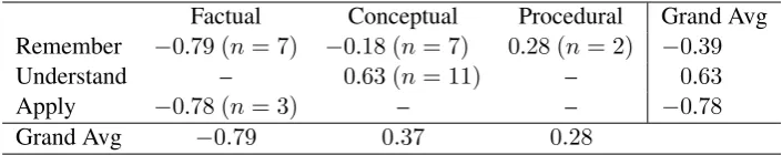
Table 4 shows the category difficulty means across both Bloom dimensions. Where the table cells are appropriately filled, the mean difficulties reflect the assumptions of the Taxonomy:

CP Remember questions are a lot easier than CP Understand questions (recall the coefficient esti-mates in Table2). Within the Remember dimension (the only one to use all three Knowledge levels), mean difficulty rises monotonically in accord with the Knowledge dimension definition.

We now see that the reason for Apply questions overall appearing twice as easy as Remember ques-tions may be the lack of Apply quesques-tions using Conceptual and Procedural knowledge. This seems more likely than an effect of noise, since all three

Apply questions are at most of difficulty−0.5, with an average of−0.78, which is clearly on the easy side of the spectrum.

It is also striking that there is an effect of CP level beyond Knowledge dimension for Con-ceptual, but not Factual questions: The Apply-Factual questions are as difficult on average as the Remember-Factual questions, while the Understand-Conceptual questions are much harder than the Remember-Conceptual questions. Fur-ther investigation with a larger data base and more closely standardized Knowledge level annotation would certainly be interesting given this pattern.

In the Knowledge Dimension grand averages, the Taxonomy is clearly mirrored: Questions us-ing Factual knowledge are easier than questions using Conceptual knowledge (this corresponds to the model coefficients shown in Table 3 above). Questions for Procedural knowledge (with annof just2) appear overall a little too easy. Keep in mind, though, that the level annotations for the Knowl-edge dimension must be assumed to be noisy given the low inter-annotatorκvalues.

In sum, both dimensions of Bloom’s Taxonomy taken together categorize the CSSAG questions into four categories of monotonously increasing difficulty in the raw data (ignoring for the moment the Apply-Factual category): Remember-Factual, Remember-Conceptual, Remember-Procedural and Understand-Conceptual. The data confirm that Bloom categories are predictive of question dif-ficulty before testing, allowing teachers and test creators to balance their tests before or even with-out norming. Vitally, however, the instructional context of the question has to be taken into account for categorization.

4 Answer Variation

Our analyses so far have looked at predicting ques-tion difficulty solely from properties of the quesques-tion (and instructional context), prior to testing. Once the question has been answered, but before grad-ing, another potentially informative predictor of question difficulty becomes available: Answer vari-ation, measured either as the average similarity of student answers among themselves or their average similarity with the reference answer.

Factual Conceptual Procedural Grand Avg Remember −0.79 (n= 7) −0.18 (n= 7) 0.28 (n= 2) −0.39

Understand – 0.63 (n= 11) – 0.63

Apply −0.78 (n= 3) – – −0.78

Grand Avg −0.79 0.37 0.28

Table 4: Cognitive Process text&question and Knowledge dimensions, Rasch difficulty averages (number of questions).

Model AdjustedR2 _{Model Sig.}

KD + CP text & question 0.290 *

Avg. SAV 0.246 *

SAV + KD + CP text & question 0.312 *

Table 5: Difficulty predicted by the Bloom Knowledge dimension (KD) and Cognitive Process (CP) levels and SAV (student answer variation): Linear modelR2 _{values and significances. *:p <0.05.}

students know. This should lead to many highly similar student answers (mirroring the reference an-swer). Difficult questions that require understand-ing of conceptual knowledge should show higher variation in the phrasing of the correct answer as well as more incorrect answers, leading to higher answer variation both among student answers and with regard to the reference answer.

If such a link indeed exists, then discrepancies between a question’s intended difficulty and its ob-served answer variation would help identify prob-lematic questions even before grading.

We model average student answer variance through the Greedy String Tiling (GST) similar-ity measure (Wise,1996), which ranges between

0 and 1 (where 0 indicates no overlap between the strings – high variation, and 1 indicates per-fect overlap – low variation). Comparing the (non-empty) student answers and the reference answer is straightforward. For the average similarity within all non-empty student answers, we use each student answer in turn as the point of comparison since GST is non-symmetric. We use the same corpus as before (see Section3.1).

Rasch question difficulty (the assumed ground truth) is indeed correlated with the average vari-ation between student and reference answers at Spearman’sρ = −0.372, p < 0.05 and with the average variation of student answers among them-selves at Spearman’sρ=−0.668, p <0.001. For both measures, difficulty is low when answer sim-ilarity is high (and therefore, answer variation is low). Perhaps surprisingly, the variation of answers among themselves is a much stronger predictor

than variation with regard to the reference answer. This may be because the similarity measure does not account for valid paraphrases (e.g., by technical terms in the reference answer). Relying just on the student answers is more elegant in any case, as no assumptions are made about the quality (or even existence) of the reference answer.

Next, we train a linear model predicting diffi-culty, just as before, but using student answer varia-tion (SAV) as a factor. Table5compares the results for SAV to a model using the Bloom KD and CP text&question levels. We also combine SAV and both Bloom dimensions. We find that all three models significantly predict difficulty. Atn= 30, there were no significant differences between the models in an ANOVA. We do see some indication of differences between the models in theR2_values, however, which reflect how much of the variance in the variabledifficultythe model accounts for. For the combination of the Bloom dimensions,R2 _is somewhat higher than for SAV alone, but combin-ing all factors yields another small increase.

We conclude that the Bloom levels, if known, are the best predictors of question difficulty. However, it can be difficult to assign the levels for existing questions if instructional materials are not available. In this case, the amount of within-answer variation for each question can be used to estimate ques-tion difficulty before grades and PTT estimates are available, or if the PTT assumptions are not met.

taxonomy categories worked better than Bloom categories. Note that they had no information on the instructional materials used and so could not adjust the CP categories (see Section3.3).

5 Automated Grading: Features and Difficulty

Having looked at difficulty and its predictability from the point of view of test creation in the pre-vious section, we now turn to an analysis of the usefulness of question difficulty information for automated grading.

In Pad´o (2016), we found that on the corpus level, there are optimal feature combinations for dif-ferent data sets. Learner corpora of text comprehen-sion questions (lower on the Bloom hierarchy) can be graded well with shallow features close to the string level, while corpora for content assessment of native speakers (containing questions higher on the Bloom hierarchy) require features derived from syntactic and semantic analysis. Following this lead, we investigate the link between question dif-ficulty and optimal feature sets for grading on the question level. We show that question difficulty can indeed be used for question-level model selec-tion (of the optimal feature set). Since quesselec-tion difficulty is often not known at grading time, we also look at Bloom’s Taxonomy levels and SAV as predictors for model selection.

5.1 Automated Grading Model and Features

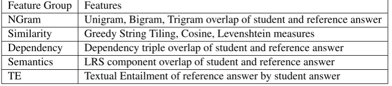
For reasons of comparability, we use the automated binary grading model fromPad´o(2016). It consists of a decision tree algorithm that considers features from five feature groups. Table6lists them in order of increasing complexity of the linguistic analysis necessary to compute them. We will refer to the NGram as well as the Similarity features (consist-ing of the Greedy Str(consist-ing Til(consist-ing, Cosine, and Leven-shtein Edit Distance similarity algorithms) as shal-lowfeatures, because only the character strings of the answers and possibly lemmatization are needed. Thedeepfeatures are the overlap between student and reference answer in terms of Dependency re-lations or Lexical Resource Semantics (LRS) com-ponents (Richter and Sailer,2004), as well as the output of the Excitement Open Platform Textual Entailment system (Magnini et al.,2014).

5.2 Method

We train the grading model in the leave-one-question-out setting on the CSSAG corpus (Sec-tion 3.1). This means the test questions and an-swers are completely unseen during training. We do five training and test runs for each question: First with only the NGram features, then adding the Similarity features and so on, until the full fea-ture set is used. We then determine for each ques-tion which feature sets yield the best performance. We report per-question prediction accuracy, which ranges between 50 and 88.9%.

5.3 Feature Sets and Model Selection

We find that for 12 out of the 30 available questions, the best performance is only reached using deep features in addition to the shallow features. For the remaining 18 questions, the best performance is already reached using just the NGram or NGram and Similarity features. In seven of these 18 cases, model performance even declines when the deep features are added, for the remaining 11 cases, ei-ther feature set yields optimal performance. These results show that there is room for question-level feature optimization.

The short-answer grading model with the full feature set (the best choice for the corpus accord-ing to Pad´o(2016)) reaches an overall accuracy of 73.11%. If we choose the best-performing fea-ture set for each question instead of the full model, overall accuracy increases to 74.35%.

These results indicate that automatic grading can be improved by choosing the best-performing grad-ing model for each question instead of relygrad-ing on a per-corpus choice. We expect greater improve-ments with fine-tuned features, because the feature implementations fromPad´o (2016) were left in-tentionally vanilla so the results would generalize more easily over the range of corpora used there.

5.4 Model Selection by Difficulty

Feature Group Features

NGram Unigram, Bigram, Trigram overlap of student and reference answer Similarity Greedy String Tiling, Cosine, Levenshtein measures

Dependency Dependency triple overlap of student and reference answer Semantics LRS component overlap of student and reference answer TE Textual Entailment of reference answer by student answer

Table 6: Overview of the feature set for automated grading

Accuracy Frequency Baseline 63.2 Difficulty 78.9

Table 7: Model Selection: Accuracy of predicting the best-performing feature set

We now change tasks and evaluate the useful-ness of difficulty for model selection. We evaluate how well the best-performing feature set (shallow or deep) for each question can be predicted by a logistic regression model (R cv.glm) using dif-ficulty as its only feature.5 _{We use leave-one-out} cross-validation.

Table7shows the classification accuracy of pre-dicting when the shallow feature set will outper-form the deep feature set. Using only ground-truth difficulty, the prediction is correct for roughly 80% of the 19 questions. This clearly outperforms the frequency baseline (always predict the deep feature set). Difficulty therefore is very informative with regard to the most useful features for SAG.

5.5 Model Selection: Bloom Levels and SAV If difficulty estimates are not available, Bloom levels or SAV may still be obtainable. We have shown above that both can be used to predict dif-ficulty. In the case of Bloom levels, we also see a promising pattern in the raw data: There is a clear tendency for questions low on the Bloom hierarchy to be optimally gradable with shallow features, while questions higher on the Bloom hier-archy require deep features. For three out of four Remember-Factual questions (out of the 19 ques-tions with one optimal feature set), optimal grad-ing performance is reached with shallow features. For the five Remember-Conceptual questions, two show optimal performance with shallow and three with deep features. Six out of seven

Understand-5_{Note that our result is strictly speaking an upper bound,} since difficulty was originally inferred using all questions.

Conceptual questions require deep features, and there is one Remember-Procedural question, also optimally graded with deep features. (The two Apply-Factual questions are split between deep and shallow features, in keeping with their estimated difficulty, see Section3.5).

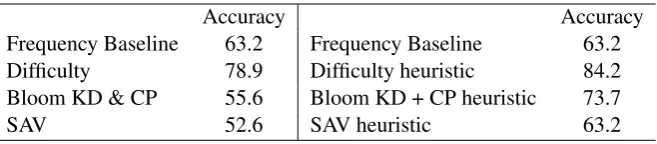
We therefore use the Bloom levels to train a logistic regression models to predict the optimal feature set, just as above. A second model uses SAV. The left-hand side of Table 8 shows that for our small data set, these factors perform practically at chance level, much below the frequency baseline.6 This pessimistic result is not the whole picture. We also evaluate three simple, conservative heuris-tics based on the Taxonomy, SAV and difficulty, respectively, that do not require training. The re-sults are on the right-hand side of Table8.

The Bloom heuristic predicts the shallow feature set for all Remember-Factual questions, and the deep feature set otherwise. Its accuracy of 74% clearly outperforms the frequency baseline.

The SAV heuristic predicts the shallow feature set for the 20% of questions with the lowest stu-dent answer variation (i.e., highest within-answer similarity). We chose 20% for the boundary based on the observation that there are five Bloom di-mension combinations present in the data and the Bloom heuristic assigns the shallow feature set for only one of them. The SAV heuristic performs at the level of the frequency baseline.

The difficulty heuristic predicts the shallow fea-ture set for the easiest 20% of questions. At 84% accuracy, this prediction model even outperforms the linear difficulty model from Section5.4.

The results underscore the usefulness of diffi-culty for model selection. In parallel to Sections3 and4above, we find that difficulty can be approxi-mated well by the levels of the Bloom Taxonomy,

Accuracy Accuracy Frequency Baseline 63.2 Frequency Baseline 63.2 Difficulty 78.9 Difficulty heuristic 84.2 Bloom KD & CP 55.6 Bloom KD + CP heuristic 73.7

SAV 52.6 SAV heuristic 63.2

Table 8: Model Selection: Accuracy of predicting the best-performing feature set. Left: Logistic model, right: Heuristic

and to a degree by the variation within student an-swers, if the levels are not available. While for small data sets such as ours, learning a selection model may not be possible, difficulty and its stand-in measures contastand-in sufficient stand-information to for-mulate an informative, yet simple heuristic model.

6 Discussion and Conclusions

Question difficulty is important in test creation and question analysis (as our discovery and exclusion of an unsuitable question in Section 3.1 demon-strates). We have shown that is also an informative factor in optimizing automated grading: Question difficulty quite accurately predicts which feature set allows best grading performance. This insight al-lows us to use question difficulty to tailor models to specific questions and optimize SAG performance.

Difficulty, however, can only be estimated af-ter grading, making it impractical to use in many SAG settings. We have shown that difficulty can be approximated by the question’s levels on Bloom’s Taxonomy, a standard tool in education, or, to a somewhat lesser extent, by SAV, the amount of variation present in student answers, measured in string similarity. These approximations are avail-able before testing (Bloom) and grading (SAV).

In this context, we can refine the hypothesis put forward in Pad´o (2016) that the grading perfor-mance variation of different feature sets over dif-ferent corpora is primarily due to differences in answer variation.Pad´o(2016) attributes these dif-ferences to different student populations (language learners have less ability to paraphrase than native or near-native speakers), which co-varied with elic-itation tasks (learner reading understanding versus native content assessment). Our results here zoom in on native-level speakers in content assessment. We found a strong relationship between preferred grading features and question difficulty, while diffi-culty is partially expressed in answer variation.

The link between Bloom hierarchy levels and dif-ficulty that we found provides more insight:

Ques-tions low on the Bloom hierarchy tend to be eas-ier and are optimally graded with shallow features (close to the text level). Questions higher on the Bloom hierarchy require deep features (more exten-sive syntactic and semantic analysis). This matches the corpus-level results fromPad´o(2016) (on top of the effect of language ability): The corpora best graded with shallow features were learner corpora of text comprehension questions. Most of these questions are low on the Bloom hierarchy, since they ask the reader to repeat knowledge explicitly presented in the text.7 _{On the other hand, content} assessment corpora (such as CSSAG) contain more and higher Bloom levels and therefore more ques-tions that require deep processing for grading.

An avenue for future work is theautomatic in-ference of Bloom Taxonomy levels. In addition to facilitating SAG, knowing question difficulty lev-els without norming would increase the quality of manually created ad-hoc tests as well as automati-cally generated question sets. The guidelines from Anderson and Krathwohl(2014) suggest that the levels can be inferred from the question wording by Textual Entailment methods. Given the nec-essary inference steps and the patterns of human annotation consistency for the two dimensions, the Cognitive Process dimension lends itself more to automated assignment than the Knowledge dimen-sion. Finally, we have shown that it is vital to identify cases of recall of instructional materials in level prediction.

Acknowledgements

The author would like to thank Sebastian Pad´o for helpful discussions and three anonymous reviewers for their insightful comments. Jan Seedorf and Se-bastian Pad´o kindly provided Bloom annotations.

References

Lorin W. Anderson and David A. Krathwohl, editors. 2014.A taxonomy for learning, teaching and assess-ing: A revision of Bloom’s. Pearson Education. Benjamin. S. Bloom, editor. 1956. The taxonomy of

educational objectives, the classification of educa-tional goals, volume Handbook I: Cognitive Do-main. David McKay, New York.

John Cunnington, Geoffrey Norman, Jennnifer Blake, Dale Dauphinee, and D. Blackmore. 1996. Apply-ing learnApply-ing taxonomies to test items: Is a fact an artifact? Academic Medicine71(10).

Steven Downey. 2010. Test development. In Pene-lope Peterson, Eva Baker, and Barry McGaw, edi-tors,International Encyclopedia of Education, Else-vier Ltd., pages 159–165.

George Due˜nas, Sergio Jimenez, and Julia Baquero. 2015. Automatic prediction of item difficulty for short-answer questions. InProceedings of the 10th Colombian Computing Conference.

Michael Hahn and Detmar Meurers. 2012. Evaluating the meaning of answers to reading comprehension questions: A semantics-based approach. In Proceed-ings of the 7th Workshop on the Innovative Use of NLP for Building Educational Applications. pages 326–336.

Sergio Jimenez, Claudia Becerra, and Alexander Gel-bukh. 2013. Softcardinality: Hierarchical text over-lap for student response analysis. InProceedings of SemEval-2013.

Jonathan Kibble and Teresa Johnson. 2011. Are faculty predictions or item taxonomies useful for estimating the outcome of multiple-choice examinations? Ad-vances in Physiological Education35:396–401. Myo-Kyoung Kim, Rajul Patel, James Uchizono, and

Lynn Beck. 2012. Incorporation of Bloom’s taxon-omy into multiple-choice examination questions for a pharmacotherapeutics course. American Journal of Pharmaceutical Education76(6).

Bernardo Magnini, Roberto Zanoli, Ido Dagan, Katrin Eichler, G¨unter Neumann, Tae-Gil Noh, Sebastian Pad´o, Asher Stern, and Omer Levy. 2014. The Ex-citement Open Platform for textual inferences. In Proceedings of the ACL demo session.

Detmar Meurers, Ramon Ziai, Niels Ott, and Janina Kopp. 2011. Evaluating answers to reading compre-hension questions in context: Results for German and the role of information structure. In Proceed-ings of the TextInfer 2011 Workshop on Textual En-tailment. Edinburgh, Scottland, UK.

Ifeyinwa Okoye, Steven Bethard, and Tamara Sumner. 2013. Cu: Computational assessment of short free text answers - a tool for evaluating students’ under-standing. InProceedings of SemEval-2013.

Ulrike Pad´o. 2016. Get semantic with me! The use-fulness of different feature types for short-answer grading. InProceedings of COLING-2016. Osaka, Japan.

Ulrike Pad´o and Cornelia Kiefer. 2015. Short answer grading: When sorting helps and when it doesn’t. In 4th NLP4CALL workshop at Nodalida. Vilnius, Lithuania.

Georg Rasch. 1960. Probabilistic Models for Some In-telligence and Attainment Tests. Danish Institute for Educational Research, Copenhagen.

Frank Richter and Manfred Sailer. 2004. Basic con-cepts of lexical resource semantics. In Arnold Beck-mann and Norbert Preining, editors,European Sum-mer School in Logic, Language and Information 2003. Course Material I, volume 5 of Collegium Log-icum, Publication Series of the Kurt G¨odel Society, Vienna, pages 87–143.

Md Arafat Sultan, Cristobal Salazar, and Tamara Sum-ner. 2016. Fast and easy short answer grading with high accuracy. InProceedings of NAACL-HLT 2016. pages 1070–1075.

Amy Tiemeier, Zachary Stacy, and John Burke. 2011. Using multiple choice questions written at various Bloom’s taxonomy levels to evaluate student perfor-mance across a therapeutics sequence. Innovations in Pharmacy2(2).

Wim van der Linden. 2010. Item response theory. In Penelope Peterson, Eva Baker, and Barry Mc-Gaw, editors,International Encyclopedia of Educa-tion, Elsevier Ltd., pages 81–88.

Michael J. Wise. 1996. YAP3: Improved detection of similarities in computer program and other texts. InSIGCSEB: SIGCSE Bulletin (ACM Special Inter-est Group on Computer Science Education). ACM Press, pages 130–134.