doi:10.1093/imanum/drh023
Advance Access publication 21 January 2005
A test problem for molecular dynamics integrators
P. F. TUPPER†
Department of Mathematics and Statistics, McGill University, Montr´eal, Qu´ebec, Canada H3A 2K6
[Received on 18 March 2003; revised on 1 June 2004]
We derive a test problem for evaluating the ability of time-stepping methods to preserve the statistical properties of systems in molecular dynamics. We consider a family of deterministic systems consisting of a finite number of particles interacting on a compact interval. The particles are given random initial conditions and interact through instantaneous energy- and momentum-conserving collisions. As the number of particles, the particle density, and the mean particle speed go to infinity, the trajectory of a tracer particle is shown to converge to a stationary Gaussian stochastic process. We approximate this system by one described by a system of ordinary differential equations and provide numerical evidence that it converges to the same stochastic process. We simulate the latter system with a variety of numerical integrators, including the symplectic Euler method, a fourth-order Runge–Kutta method, and an energy-conserving step-and-project method. We assess the methods’ ability to recapture the system’s limiting statistics and observe that symplectic Euler performs significantly better than the others for comparable computational expense.
Keywords: equations and systems with randomness; Hamiltonian systems; statistical mechanics; symplectic numerical methods.
1. Introduction
In the field of molecular dynamics, researchers use numerical integrators to approximate the motion of systems of particles. They integrate over long periods of time and extract statistical information from the computed trajectories. This, in turn, can be used to determine the macroscopic properties of the system. For optimal efficiency, the researchers integrate using as long a step-length as possible while still maintaining the stability of the computed solution. In this regime, trajectories are not computed accurately. Nevertheless, it is observed that statistical features of solutions are maintained in some circumstances. (See Allen & Tildesley, 1989; Deuflhardet al., 1999.)
One possible explanation for this phenomenon is the existence of an underlying stochastic process (Sigurgeirsson & Stuart, 2001). Suppose that the trajectories of the deterministic process approximate some stochastic process in the sense of distribution. If we use a numerical method whose trajectories also approximate the same stochastic process, then the numerical solution will have similar statistical features to the original system, even though there is no path-wise agreement.
The goal of this paper is to construct a test case for this situation. We seek a deterministic system having a component of its trajectory that approximates a well-understood stochastic process. Once given such a system, we can use it to test numerical integrators. We integrate the system with a numerical integrator using step-lengths that do not resolve the trajectories correctly. Then we can investigate
†Email: [email protected]
how accurately these computed solutions reproduce the statistical features of the underlying stochastic process.
Our construction is inspired by a 1968 paper by Spitzer (1968/1969) that provides an example of a sequence of deterministic systems whose trajectories converge to a stochastic process. Building on the previous work of Harris (1965), he shows that Brownian motion can be obtained as the limit of a sequence of deterministic processes on the real line with random initial conditions. His construction consists of placing point particles on the real line according to a Poisson distribution. Each particle is assigned a random velocity independently of the other particles. The particles are allowed to move, so that they interact through energy- and momentum-conserving collisions: i.e. whenever two particles meet, there is an instantaneous collision in which they exchange velocities. A single particle is placed at the origin and its subsequent trajectory observed. Spitzer proves that with an appropriate scaling of the variables, the path of this tracer particle converges weakly to standard Brownian motion.
There are two difficulties with using this system for our investigations. The first is that since it is infinite in extent, it is impossible to simulate it completely on a computer. As a way of avoiding this difficulty, in Section 2 we introduce a finite counterpart to Spitzer’s set-up. We describe a sequence of systems each consisting of afinitenumber of particles interacting on acompactsegment of the real line. In Sections 3 and 4, we prove that as the number of particles goes to infinity, the trajectory of a tracer particle will converge to a stationary Gaussian process with a known correlation function.
The second difficulty is that neither Spitzer’s system nor the system we present in Section 2 are described purely in terms of ordinary differential equations, since the inter-particle collisions are instantaneous. Thus, we cannot use these systems as test problems for numerical integrators without dealing with the issues of collision detection. However, we show, in Section 5, how we can approximate the non-differentiable flow of these systems with the flow of a differential equation by replacing the hard, instantaneous collisions of the particles with collisions mediated by a soft potential. This system approximates the non-differentiable system in the limit as the stiffness of the inter-particle forces goes to infinity. If we allow both the number of particles and the inter-particle stiffness to go to infinity with a particular scaling, we conjecture that the tracer particle’s trajectory converges to the same Gaussian process. We show the results of numerical experiments that support this statement.
In Section 6, we use the family of systems introduced in Section 5 as a test problem for a variety of time-stepping methods. We apply five different numerical methods to the system: symplectic Euler, backward Euler, forward Euler, a fourth-order Runge–Kutta method, and an energy-conserving step-and-project method. We observe that, of these methods, only the symplectic Euler and the step-and-step-and-project method are able to even approximatley reproduce statistics in the limiting case with reasonable step sizes. The latter energy-conserving method is more costly and it is not able to take longer steps than symplectic Euler without damaging its ability to recover the stochastic limit. We conclude that, for this test problem, the symplectic Euler method is clearly the superior method out of those considered here. This coincides with computational practice in molecular dynamics, where use of the Verlet integrator (a version of symplectic Euler) is ubiquitous (Allen & Tildesley, 1989).
Though our interest in simulation has led us to consider finite systems, other researchers have continued with Spitzer’s (1968/1969) ideas in different directions. One possibility is to allow the mass of the tracer to differ from the mass of the other particles. Holley (1971) proves that with such a scaling the trajectory of the tracer particle weakly converges to the Ornstein–Uhlenbeck process. M¨urmann (1973) takes this result further by proving a similar result when the collisions between the particles do not occur instantly but are mediated by a soft potential.
(1999), Hald & Kupferman (2002) and Kupferman et al. (2002) have rigorously shown stochastic limiting behaviour for the Ford–Kac heat-bath model (Ford & Kac, 1987). Like the model in the present paper, a sequence of Hamiltonian systems with random initial conditions and increasing numbers of particles is considered. In the infinite particle limit, the trajectory of the tracer particle is shown to converge to the solution of a stochastic differential equation. This construction has been used to analyse numerical integrators in Canoet al.(2001) and more sophisticated algorithms in Huisingaet al.(2003). 2. Particle systems on a compact interval
In this section, we describe a sequence of particle systems on the interval[−1,1]. For each odd positive integern, the system will consist ofninteracting particles (contrary to the convention in the interacting particle literature). We let the tracer particle be the ‘median’ particle in the interval, i.e. the one with an equal number of particles on either side of it. When we scale the interval by a factor ofn1/2, we will see that the trajectory of this tracer particle will converge to a Gaussian random process.
Let qi, i = 1, . . . ,n be independent and identically distributed (i.i.d.) random variables, each
uniformly distributed on[−1,1]. These are the initial positions of thenparticles. We give the particles i.i.d. velocities pi according to a distribution with a probability density f. We make the following
assumptions on f.
ASSUMPTIONS2.1 The probability density f satisfies (i) f is symmetric: f(−p)= f(p).
(ii) f isL1and non-trivial: 0<E|pi|<∞.
(iii) f is compactly supported:P{|pi|>Vmax} =0 for someVmax.
Note that the third condition implies that f isL1. However, we leave the assumptions in this form since some results will be proven without using condition (iii).
Given these initial conditions, we allow the particles to move according to the following rules. Particles move at constant velocity until they encounter either another particle or one of the barriers at−1 or 1. If two particles collide, they merely exchange velocities. If a particle hits a wall, it reverses its velocity. These rules are a natural consequence of assuming that the total energy of the system is conserved and that when two particles collide, their total momentum is conserved. With these rules for motion, we designate the position at timet of the particle starting atqi byxi(t). Note that the order of
the particles is unchanged in time. By this we mean that ifqi <qj, thenxi(t) xj(t)for allt 0.
Chooseimedso thatqimed is the median of the{qi}. It follows thatximed(t)is the median of the{xi(t)}for allt. We choose this particle to be our tracer particle and definexmed(t):=ximed(t)fort 0.
If we multiply the positions of all of the particles over time byn1/2, we obtain a system ofnparticles interacting over the interval[−n1/2,n1/2], with an average particle speed ofn1/2E|pi|. We will denote
the position of the tracer particle with this scaling byUn, so thatUn(t)=n1/2xmed(t)fort0.
In order to get a more convenient representation of the motion of the tracer particle, we now describe a different, but related, set of rules of motion. The rules of motion are the same as before except that the particles do not interact with each other but only with the walls. Thus, when the trajectories of two particles intersect, the particles merely pass through each other. Under this set of rules, we designate the position of the particle starting atqi byyi(t), fort 0. There is a simple expression for yi(t). If there
were no walls, the particle’s position at timetwould beqi+t pi. The effect of the walls is to ‘fold’ the
particle’s trajectory back into the interval[−1,1]. This is accomplished by a functionGsuch that
1
1 2 3 4 5
-1 -2 -3 -4
1
FIG. 1. The functionH.
Gis the periodic function with period 4 such that
G(x)=
x, −1x 1
2−x, 1x3. (2.2)
There is a relationship between the two sets of trajectories,{xi(t)}and{yi(t)}. At any point in time,
the set of positions the particles take is the same under the two different rules of motion. Since the position of the tracer particle at any time is given by the median of all thexi(t), its position is also given
by the median of all theyi(t). So the trajectory of the tracer particle is given by
Un(t):=n1/2xmed(t)=n1/2 med
i=1,... ,n(yi(t))=n
1/2 med
i=1,... ,n(G(qi+t pi)). (2.3)
This is a convenient representation, since{qi}ni=1 and{pi}ni=1are independent random variables with
known distributions.
It is straightforward to check that, for eachi,yiis a stationary stochastic process. As a consequence,
bothxmedandUnare stationary processes as well. The distribution of yi(t)is uniform on[−1,1]for
allt.
We briefly review the concept of weak convergence in a topological space. Let X be a topological space with random elementsU,Un,n 1. We say thatUnweakly converges toUand writeUn⇒U,
if for all bounded continuous functionsg : X → R,Eg(Un)→ Eg(U)asn → ∞. We will consider
two examples of X in this paper. The first isC[0,T], the space of real-valued continuous functions on
[0,T]with the topology induced by the supremum norm. The second isRdwith the standard topology. See Billingsley (1999) for a thorough exposition of weak convergence.
We now present our main result. It states that as the number of particlesngoes to infinity, the scaled trajectory of the tracer particle will converge weakly to a Gaussian process inC[0,T]. This result is the basis for the numerical experiments performed later in the paper. For the statement of the main theorem, we defineHto be a periodic function with period 4 such that
H(z)=
1−z, 0z2,
z−3, 2z4 (2.4)
as shown in Fig. 1.
THEOREM2.2 Let{qi}i1,{pi}i1, be mutually i.i.d. sequences of random variables, where eachqiis
0 1 2 3 4 5 6 7 8 9 10 –0·2
0 0·2 0·4 0·6 0·8 1
Uniform Velocity Distribution
0 0·5 1 1·5 2 2·5 3 3·5 4
–0·2 0 0·2 0·4 0·6 0·8 1
Gaussian Velocity Distribution
FIG. 2. Covariance functions for two choices of the velocity distribution.
For each odd positive integern, let
Un(t):=n1/2 med
i=1,... ,n(G(qi +t pi)).
Then, asn→ ∞,
Un(t)⇒U(t),
whereU(t)is the stationary continuous mean-zero Gaussian process with covariance C(t):=E[U(0)U(t)] =
∞
−∞H(pt)f(p)dp. (2.5)
The convergence is in the weak sense inC[0,T]for anyT >0.
We note that we will have completely determined the limiting process since a mean-zero continuous Gaussian process is completely specified by its covariance function. Since our process is stationary, we have
EU(s)U(t)=EU(0)U(t−s)=C(t−s).
Equation (2.5) gives the covarianceCas it depends on the velocity density function f. In Fig. 2, we show plots ofCversustfor two choices of f. The first shows the case when velocities are chosen uniformly in
[−1,1]; the second shows the case when they are chosen according to the standard Gaussian distribution. Alternatively, when we choose velocities to be either−1 or 1, each with probability 1/2, thenC = H defined by (2.4) and shown in Fig. 1.
4 time units. Thus, both the trajectory of the tracer particle and the covariance function itself are periodic functions of period 4.
The standard method for proving weak convergence of random processes inC[0,T]is first to show that the finite-dimensional distributions converge and then that the family of approximating processes is tight. In particular, we have the following standard result, adapted from Billingsley (1999, Theorem 7.5). We define the functionwδ,[0,T]onC[0,T]by
wδ,[0,T](U)= sup t1,t2∈[0,T],|t2−t1|<δ
|U(t2)−U(t1)|. (2.6)
THEOREM2.3 LetUn,n1,Ube processes inC[0,T]such that
(i) Finite-dimensional distributions converge: For allt1, . . . ,td∈ [0,T], we have that {Un(tj)}j=1,... ,d ⇒ {U(tj))}j=1,... ,d
asn→ ∞(i.e. weak convergence inRd).
(ii) The processes satisfy a tightness criterion: For all >0 and allη >0, there is aδ >0 such that
P{wδ,[0,T](Un)}η,
for alln. ThenUn⇒UinC[0,T].
In Section 3, we establish the convergence of the finite-dimensional distributions and, in Section 4, we establish the tightness criterion. We are able to prove the former result without the assumption of the velocity distribution being compactly supported. We conjecture that the main theorem holds without this assumption but could not obtain the tightness result without it.
Spitzer also divides his proof into proving the convergence of finite-dimensional distributions and then establishing tightness. In his case, Spitzer accomplishes the former task with the use of characteristic functions (Fourier transforms of density functions). In our case, the fact that there is a finite number of particles allows us to avoid this and appeal directly to a version of the Central Limit Theorem (CLT) for medians. Proving tightness for our family of trajectories cannot be done with Spitzer’s techniques, since his arguments rely heavily on the processes having independent increments. Instead we observe that, if velocities are bounded, over short intervals of time the tracer particle undergoes motion that approximates in distribution that of the tracer in Spitzer’s system. We are able to control this approximation sufficiently well to show that the trajectories in our system inherit the tightness of the trajectories in Spitzer’s system.
3. Convergence of finite-dimensional distributions
In this section, we establish the convergence of the finite-dimensional distributions of the tracer particles’ trajectories to those of the limiting Gaussian process. For any set of timest1, . . . ,td 0, the random
vector{Un(tj)}j=1,... ,d is the scaled median of the n i.i.d. random vectors {yi(tj)}j=1,... ,d. We wish
to show that this random vector converges weakly to the Gaussian random vector{U(tj)}j=1,... ,d as
In the proof, we use the following characterization of weak convergence inRd. For a random vector Y inRd, we define its distribution functionFY :Rd →Rby
FY(x1, . . . ,xd):=P{Y(1)x1, . . . ,Y(d)xd},
whereY(j)is the jth component ofY. We say thatx∈Rdis a continuity point of the random vectorY ifFY is continuous atx. Random vectorsYn,n1, converge weakly toYif and only if for all continuity
pointsxofY,
P{Yn(j)xj,j =1, . . . ,d} →P{Y(j)xj,j=1, . . . ,d}, (3.7)
asn→ ∞(Billingsley, 1999).
LEMMA3.1 Let the velocity density f satisfy conditions (i) and (ii) of Assumptions 2.1. Then the finite-dimensional distributions ofUn converge weakly to those ofU. That is, for anyt1, . . . ,td ∈ [0,∞),
{Un(tj)}j=1,... ,d⇒ {U(tj)}j=1,... ,d,
asn→ ∞.
Proof. Letx∈Rdbe a continuity point of{U(tj)}j=1,... ,d with componentsxj,j =1, . . . ,d. We use
the characterization of weak convergence inRdgiven in (3.7). Consider the event of interest:
{Un(tj)xj,j =1, . . . ,d} = {n1/2xmed(tj)xj,j=1, . . . ,d} = {xmed(tj)n−1/2xj,j=1, . . . ,d}.
Recall thatxmed(t)is the median ofyi(t),i =1, . . . ,n. Using a standard identity for medians, we have,
for eachj,
{xmed(tj)n−1/2xj} =
n
i=1
1yi(tj)n−1/2x j n/2
,
where1Ais the indicator function of the event A. So {Un(tj)xj} =
− n
i=1
1yi(tj)n−1/2x
j −n/2
.
Let us manipulate the event on the right-hand side of the equation. We subtract the expectation of the left-hand side of the inequality from both sides. Since
E−1yi(tj)n−1/2xj
= −
1+n−1/2xj
2
,
we obtain
{Un(tj)xj} =
n
i=1
1+n−1/2xj
2 −1yi(tj)n−1/2xj
n
i=1
n−1/2xj
2
=
n−1/2
n
i=1
[1+n−1/2xj−21yi(tj)n−1/2xj]xj
Let us define
νn,i,j :=1+n−1/2xj −21yi(tj)n−1/2xj (3.8) and
Nn,j :=n−1/2 n
i=1
νn,i,j. (3.9)
Then
{Un(tj)xj,j =1, . . . ,d} = {Nn,j xj,j =1, . . . ,d} =
n−1/2
n
i=1
νn,i,j xj,j =1, . . . ,d
.
The event on the right-hand side is now in a form amenable to a multivariate CLT. In the appendix, we show that {Nn,j}j=1,... ,d weakly converges to a Gaussian random vector with covariance matrix Σi j =C(ti −tj). Therefore,
P{Nn,j xj,j =1, . . . ,d} →P{U(tj)xj,j=1, . . . ,d}
sincexis a continuity point of{U(tj)}j=1,... ,d. This establishes the desired result.
4. Tightness criterion
Now that we have proven that the finite-dimensional distributions of Un converge to those of U, it
remains to show that the sequence of processesUnsatisfies the tightness criterion of Theorem 2.3. We
will do this by describing another construction of the processesUn. First, we will provide a construction
of the process in Spitzer’s (1968/1969) paper,Vn ∈ C[0,∞),n 1. Then we will apply a random
transformation toVnto obtain another sequence of processesUˆn, defined on the same probability space,
that also satisfies the tightness criterion. This sequence of processes will have the advantage that they are identical toUnon a certain time interval with a high probability. This will allow us to establish the
tightness criterion forUn. Our approach here is similar to that used to prove tightness in another context
in D¨urret al.(1980/81).
We now describe one possible construction of Spitzer’s processes. For each oddn 1, we place particles on the real line according to a uniform Poisson process with constant densityn/2. We add a tracer particle at the origin. We denote the particle positions with. . .z−2z−1z0=0z1z2. . .. We give the particles i.i.d. velocitieswj from the density f. The motion of the particles is the same as
for our system but without walls: instantaneous momentum- and energy-conserving collisions with free motion otherwise. At timest 0, we multiply the position of the tracer particles byn1/2to getVn(t).
A more formal definition ofVnis
Vn:=n1/2 lim
p→∞ i=−medp,... ,p(zi +twi),
which is shown in Harris (1965) to agree with the previous physical definition. Spitzer’s paper proves that Vnweakly converges to Brownian motion (with some non-random constant scaling in time). The result of
of Theorem 2.3 is satisfied by them (Billingsley, 1999). Moreover, the set of velocity distributions for which Spitzer obtains his result contains the set of distributions that satisfy Assumptions 2.1.
We now make some comments about the initial inter-particle spacing in this system. Recall that for a uniform Poisson process on the real line, the inter-particle spacings are i.i.d. exponential random variables. Indeed, the addition of the tracer particle at 0 does not change this fact (Spitzer, 1968/1969). If we defineξi =zi−zi−1for alli, theξi are i.i.d. exponential random variables with mean 2/n.
Each processVnis defined on a probability space of bi-infinite sequences({zi},{wi}). For each odd
n we shall define a new processUˆn(t)on the same space. Letm = (n−1)/2. We define the random
variables
ρn=
zm+1−z−m−1
2 , µn=
zm+1+z−m−1
2 .
Note that
ρn=
1 2
m+1
i=−m
ξi, Eρn=
n+1
n . (4.10)
We let
ˆ
zi =(zi−µn)/ρn (4.11)
for alli. We have performed an affine transformation to the positions of the particles so thatzˆm+1=1 andˆz−m−1= −1. Now, with probability one, there are exactlynparticles in the open interval(−1,1). We defineUˆnas we didVnbefore but with the initial particle positions{ˆzi}. So
ˆ
Un(t):=n1/2 lim
p→∞ i=−medp,... ,p(ˆzi+twi). (4.12)
Using (4.11) and (4.12) we can obtain an explicit relationship between the two sequences of processes. For eachn,
ˆ
Un(t)=n1/2 lim
p→∞ i=−medp,... ,p((zi −µn)/ρn+twi) =ρ−1
n n1/2
lim
p→∞ i=−medp,... ,p(zi +(ρnt)wi)−µn
= [Vn(ρnt)−n1/2µn]/ρn.
Using this relation we now establish that the family of processes satisfies the tightness criterion.
LEMMA4.1 The sequence of processes Uˆn(t), n 1, n odd, satisfies the second condition of
Theorem 2.3 inC[0,T]for anyT >0.
Proof. Let us fix an interval[0,T]. Recall the definition ofwδ,[0,T]from (2.6). First note that
wδ,[0,T](Uˆn)= sup t1,t2∈[0,T],|t1−t2|<δ
| ˆUn(t2)− ˆUn(t1)|
= sup
t1,t2∈[0,T],|t1−t2|<δ
|Vn(ρnt2)−Vn(ρnt1)|/ρn
= sup
ˆ
t1,tˆ2∈[0,ρnT],|ˆt1−ˆt2|<ρnδ
|Vn(t2ˆ)−Vn(t1ˆ)|/ρn =ρ−1
where we have used the substitutiontˆ=ρnt. Now let us fix an >0 and anν >0. We have that
P{wδ,[0,T](Uˆn)} =P{ρn−1wρnδ,[0,ρnT](Vn)}
P{ρn∈ [1/2,2]} +P{w2δ,[0,2T](Vn)/2}.
By (4.10) and the law of large numbers,ρnconverges almost surely to 1. So we can choosen1such that
nn1implies that the first probability is less thanν/2. By the tightness ofVn, we can find ann2and aδ
such that the second term is less thanν/2 for allnn2. ChoosingN =max(n1,n2)gives the required
result.
Our reason for introducingUˆnis that the positionszˆ−m, . . . ,zˆm are now distributed identically to
the order statistics of the positionsq1, . . . ,qnof our original system described in Section 2. To see this,
note that we can write thezˆi as ˆ
z−m−1+j =(z−m−1+j−µn)/ρn =
z−m−1+
−m−1+j
i=−m
ξi
−(z−m−1+zm+1)/2 ρn
= −1+2
−m−1+j
i=−m
ξi
m+1
i=−m
ξi
.
Since the ξi are i.i.d. exponential random variables, the ratio of the sums of theξi in the previous
expression for j =1, . . . ,n are distributed as the order statistics ofn i.i.d. uniform random variables on[0,1](Durrett, 1996, p. 148). Soˆz−m−1−j for j =1, . . . ,nare distributed as the order statistics of
ni.i.d. uniform random variables on[−1,1].
This gives us a way of defining our original processUn on the same space as Vn andUˆn. Before
we definedUn(t)=medi=1,... ,nG(qi+pi)whereqi were i.i.d. uniform random variables on[−1,1].
However, since thepi are distributed independently of theqi, this is identical in distribution to defining
Un as medi=1,... ,nG(q[i]+pi)whereq[j]is the jth order statistic of theqi. Therefore, we can define
Unby
Un(t)= med
i=−m,... ,mG(zˆi+wit).
Physically, this has the following interpretation. To generate the random trajectoryUn, we set up the
particles as we did forUˆn. But now we remove all but thenparticles with positionszˆ−m, . . . ,ˆzm(which
are all in[−1,1]) and add walls at−1 and 1. We then let the particles move and interact with each other and with the walls as before. The trajectory of the tracer particle multiplied byn1/2gives usUn. The
trajectory of the particles will be different forUnandUˆn. However, since particle speed is bounded by
Vmaxaccording to Assumption 2.1(iii), there will be a period of time during which, with high probability,
the trajectory of the tracer will not be affected. This is the content of the following theorem.
LEMMA4.2 The probability thatUˆnandUnare identical on the time interval[0,1/4Vmax]goes to one
asn→ ∞.
from the walls at time 0 it will not be able to distinguish the difference between the set-ups forUˆnand
Unfor that interval of time, and the two processes will be identical. Now,
P{ˆz0>1/2} =P
med
i=1,... ,nqi >1/2
=P
i=1,... ,n
1qi>1/2>n/2
=P
n−1
i=1,... ,n
1qi>1/2>1/2
.
Since theE{1qi>1/2} =P{qi >1/2} =1/4, the probability in question converges to 0 asn → ∞by
the law of large numbers.
With these two lemmas, we can establish the tightness result.
THEOREM4.3 The family of processesUn(t),n 1 satisfies the second criterion of Theorem 2.3 in
C[0,T]for anyT >0.
Proof. Fix aT >0. Let, ν >0 be given. LetMbe an integer such thatM/4VmaxT. For anyδ >0, wδ,[0,T](Un)wδ,[0,M/4Vmax](Un)
2 max
i=1,... ,Mwδ,[(i−1)/4Vmax,i/4Vmax](Un).
SinceUnis a stationary process,wδ,[(i−1)/4Vmax,i Vmax/2](Un)has the same distribution regardless ofi. So
P{wδ,[0,T](Un)}
i=1,... ,M
P{wδ,[(i−1)/4Vmax,i Vmax/2](Un)/2M} =MP{wδ,[0,1/4Vmax](Un)/2M}.
This last probability is less than or equal to
P{Un≡ ˆUnon[0,1/4Vmax]} +P{wδ,[0,1/4Vmax](Uˆn)/2M}.
The first term can be made less thanν/2 by choosingnn1for somen1, by the previous lemma. Since
ˆ
Un is tight, we can choose aδ > 0 and ann2such that the second term is less thanν/2 forn n2.
Using thisδandN=max(n1,n2)gives us the result we need forUn.
5. Approximation with soft collisions
We have now shown that a particular sequence of deterministic processes with random initial conditions has a componentUn, defined by (2.3), that converges to a mean-zero Gaussian processU specified by
As before, for each odd positive integer n, we place n particles independently on the interval
[−n1/2,n1/2]according to a uniform distribution. Each particle is independently given a velocityn1/2p wherepis selected from the distribution with density f, as before. The two choices of f we will consider are (i) standard normal distribution and (ii) uniform on[−1,1]. Though our main convergence theorem does not apply in case (i), the convergence of the finite-dimensional distributions does and that is what we shall consider in our experiments. We denote the position and velocity of particleiat timetbyqi(t)
and pi(t)respectively, withqi+1(0) > qi(0). In contrast to the previous case, we describe the motion
of the particles through a set of ODEs. The differential equations describing the positionsqi and the
momentapi are
˙
qi(t)= pi(t), i =1, . . . ,n,
and
˙
p1(t)= −k2(q1(t)−q2(t))++k2(−n1/2−q1(t))+,
˙
pi(t)= −k2(qi(t)−qi+1(t))++k2(qi−1(t)−qi(t))+, i=2, . . . ,n−1, ˙
pn(t)= −k2(qn(t)−n1/2)++k2(qn−1(t)−qn(t))+,
where (x)+ = max(0,x) for x ∈ R. This system can be viewed as a Hamiltonian system with Hamiltonian
H(q,p)=V(q)+1 2
n
i=1
pi2, (5.13)
where
V(q)= 1 2k
2(−n1/2−q1)2
++12 n−1
i=2
k2(qi−1−qi)2++
1 2k
2(q
n−n1/2)2+. (5.14)
The tracer is chosen as the particle with the median position at time zero.
The flow of this system of ODEs is very similar to that of the original process. However, when two particles meet each other, rather than instantaneously exchanging velocities, they are allowed to overlap. While overlapping, they apply a repelling force to each other that is proportional to the amount that they have overlapped. Thus, while the particles are in contact, they go through simple harmonic motion. After half a period of this motion, they cease to overlap and have velocities pointing away from each other. Since momentum and energy are conserved, the net effect is that their velocities are exchanged, as in the hard collision case. However, their positions are displaced relative to where they would be after a hard collision. This only describes a two-particle collision: collisions with three or more particles occur with non-zero probability and are more complicated.
In the previous ODEs,kis a constant denoting the stiffness of the repulsion between the particles and between the particles and the walls. Fork =0, the particles do not interact at all; ask → ∞, we expect the trajectories of the system to converge to those of the original system with the same initial data. (See, for example, Paoli & Schatzman, 1993 or Turaev & Rom-Kedar, 1998.)
collisions and, in the limit ofn → ∞, we expect the system to be a close approximation to the system with instantaneous collisions. We conjecture that the ODE system, with this choice ofk, has the same limiting properties as those we proved for the instantaneous collision system: the trajectory of the tracer particles weakly converges toU. We believe this holds true for all positiveγ, though in the following we fixγ =1. We now provide some numerical evidence to support this conjecture in this case.
As before, C is the covariance of the limiting processU which depends on f. Define Cn to be
the covariance of our original hard-particle process withn particles described in Section 2. Our main theorem in Section 3 shows thatCn(t)converges toC(t)for allt for both choices of f given earlier.
We denote byCn,k the covariance function for the process described by the ODEs withnparticles and
a stiffness parameterk. A consequence of the softened system converging weakly toU as n → ∞ withk = n2 would be the convergence ofCn,k toC. For a givenn,k, the natural way to obtain an
accurate approximation toCn,kwould be to simulate the system numerically with a time step so small
that trajectories are accurately computed over the time interval of interest. We would expect that steps of size∆t = o(1/k) = o(1/n2) would be required for this. Unfortunately, this is impractical for larger values ofn. Instead, let us defineCn,k,∆t to be the autocovariance function for the numerical
approximation to the system withnparticles, stiffness parameterkand integration step-length∆t. We will computeCn,k,∆t for diminishing values of∆t until we observe convergence. This converged value
we will take as our estimate toCn,k. In this section, we will exclusively use the symplectic Euler method,
given by the formulae:
qn+1 = qn+∂H/∂p(qn,pn),
pn+1 = pn−∂H/∂q(qn+1,pn+1), (5.15)
whereHis given by (5.13) and (5.14). This is explicit in our case since∂H/∂q does not depend onp. We demonstrate this procedure for the Gaussian velocity distribution in Fig. 3. Forn = 3,15,75 withk=n2, we showCn,k,∆t −Cnfor a range of∆t. We subtract the functionCnso that it is easier
to see the differences betweenCn,k,∆t for different∆ton one graph. (Note that the scale on they-axis
differs in each plot.) For eachn,Cn,k,∆t appears to converge as∆t →0 within the accuracy provided
by our statistics. Moreover, convergence is attained with a step-size of∆t >1/2k. Similar results were found for the uniform velocity distribution as we show in Fig. 4. Accordingly, we take results computed with symplectic Euler with the step-size∆t =1/2kto be accurate estimates ofCn,k for both velocity
distributions.
To show thatCn,kconverges toCwithk=n2, we take these estimated values and plot the difference
C−Cn,k,∆t,∆t =1/2k, for varyingn. Figure 5 shows that the difference appears to converge to zero
for both velocity distributions, though this is less clear in the case of the uniform velocity distribution. Of course, convergence of the covariance function does not guarantee convergence of the process but the evidence partly confirms our hypothesis.
0 0·2 0·4 0·6 0·8 1 1·2 1·4 1·6 1·8 2 –0·02
0 0·02 0·04 0·06 0·08 0·1 0·12 0·14 0·16
n=3, k=n2
∆t = 0·12
∆t = 0·06
∆t = 0·03
0 0·2 0·4 0·6 0·8 1 1·2 1·4 1·6 1·8 2
–0·01 0 0·01 0·02 0·03 0·04
n=15, k=n2
∆t = 0·0045
∆t = 0·00225
∆t = 0·001125
0 0·2 0·4 0·6 0·8 1 1·2 1·4 1·6 1·8 2
–0·04 –0·03 –0·02 –0·01 0 0·01 0·02 0·03
n=75,k=n2
∆t = 0·0001
∆t = 0·00005
∆t = 0·000025
FIG. 3.Cn,k,∆t−Cnfor three choices ofn,k, for a range of∆twith the Gaussian initial velocity distribution. On the first graph
the standard deviation of the error is approximately the thickness of the lines; on the second and third representative error bars are shown.
6. Numerical approximation
In the previous section, we presented a sequence of particle systems described by ODEs and parametrized byn, the number of particles, andk, the stiffness of the collisions. If we let k = n2, it appears that the trajectory of the tracer particle weakly converges to that of the stochastic processU as ngoes to infinity. Moreover, when the system was integrated with the symplectic Euler method with a large step-size (∆t = 1/2k), the same stochastic limit was obtained. In this section, we will examine how other methods perform in comparison.
For any given numerical integrator, as we increasen(and thusk), it is necessary for∆tto be reduced in order to capture any features of the system. Since the duration of time two particles spend colliding is of order 1/k, to have an integrator take at leastsome steps during each collision as n → ∞, it is necessary that∆t = O(1/k)or smaller. We have already seen that symplectic Euler captures the limiting statistics with this scaling. For a method to be competitive with the symplectic Euler near the stochastic limit, it must have∆t = O(1/k)as well. (Indeed, we expect that if∆t goes like 1/kd for d > 1, then all convergent methods will capture statistics well on finite time intervals in the limit.) Accordingly, we shall test all methods with step-length∆t =γ /kfor someγ >0.
0 0·2 0·4 0·6 0·8 1 1·2 1·4 1·6 1·8 2 0
0·05 0·1 0·15
n=3, k=n2
∆t = 0.12
∆t = 0.06
∆t = 0.03
0 0·2 0·4 0·6 0·8 1 1·2 1·4 1·6 1·8 2
–0·01 0 0·01 0·02 0·03 0·04 0·05
n=15, k=n2
∆t = 0·0045
∆t = 0·00225
∆t = 0·001125
0 0·2 0·4 0·6 0·8 1 1·2 1·4 1·6 1·8 2
–0·05 –0·04 –0·03 –0·02 –0·01 0 0·01 0·02 0·03
n=75, k=n2
∆t = 0·0001
∆t = 0·00005
∆t = 0·000025
FIG. 4.Cn,k,∆t−Cnfor three choices ofn,k, for a range of∆twith the uniform initial velocity distribution. On the first graph
the standard deviation of the error is approximately the thickness of the lines; on the second and third representative error bars are shown.
we will examine how each method performs computing individual trajectories of the system for three values ofn. We conclude in Section 6.3 by examining how the symplectic Euler method and its projected version fare at capturing the limiting statistical behaviour of the system.
6.1 Numerical methods
We consider five numerical methods all used with a constant stepsize. The first is the symplectic Euler method as given in (5.15). The second and third are standard methods, the backward and forward Euler. The fourth is a fourth-order Runge–Kutta method (Haireret al., 1987), with Butcher tableau
0 1 2
1 2 1
2 0
1 2
1 0 0 1
1 6
2 6
2 6
1 6
0 0·2 0·4 0·6 0·8 1 1·2 1·4 1·6 1·8 2 –0·1
–0·05 0 0·05 0·1 0·15 0·2 0·25 0·3 0·35 0·4
C
(
t
)–
Cn
(
t
)
t
Gaussian Velocity Distribution
n=3
n=15
n=75
0 0·2 0·4 0·6 0·8 1 1·2 1·4 1·6 1·8 2
–0·1 0 0·1 0·2 0·3 0·4
C
(
t
)–
Cn
(
t
)
t
Uniform Velocity Distribution
n=3
n=15
n=75
FIG. 5.C(t)−Cn,k,∆t(t)fort∈ [0,2]withk=n2,∆t=1/2kfor both velocity distributions considered. The standard deviation
of the error on the curves never exceeds 0·004.
One property of the symplectic Euler method which may be viewed as a drawback for molecular dynamics simulations is that it does not conserve the energy of the system exactly. One way to remedy this is to use a step-and-project method; see Haireret al.(2002, IV.4). A step-and-project method is a modified version of a standard time-stepping algorithm wherein the solution is forced to have the correct energy after each step. This is done by first taking a step with a standard method—which will lead to a value with possibly incorrect energy—and then projecting this value onto the manifold of states with the correct energy.
Typically, step-and-project methods for Hamiltonian systems are implemented as follows. Suppose we are numerically integrating a Hamiltonian system of ODEs on the space of pointsx=(q,p)∈R2n with fixed energyH(x) = H0. From a state xn = (qn,pn)with the correct energy, a standard
time-stepper is used to obtain the state xn∗+1. The gradient of the Hamiltonian is computed at this state: s= ∇H(x∗n+1). Then anα∈Ris computed so thatH(xn∗+1+αs)=H0. Then we setxn+1=xn∗+1+αs. (In our case anαwas determined so that|H(xn+1)−H0|<10−5.)
In our implementation there are two aspects of this scheme that we modify. First, the we use a different projection directions. The usual choice,
s= ∇H(q,p)=[∇V(q) p]T, does not scale well with increasingk. Instead we use
s=
∇V(q) k2p
T
.
0 0·5 1 1·5 2 2·5 3 3·5 4 –2
–1 0 1 2
0 0·5 1 1·5 2 2·5 3 3·5 4
–4 –2 0 2 4
0 0·5 1 1·5 2 2·5 3 3·5 4
–10 –5 0 5 10
FIG. 6. Trajectories computed with the symplectic Euler method with∆t =1/k. Plots are of particle position versus time for
n=3,15,75,k=n2.
6.2 Single trajectories
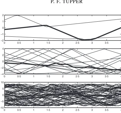
Before we consider these methods’ ability to reproduce the stochastic limit, we will first examine the performance of each method on a single trajectory of the model system withn=3,15,75 andk=n2, as in the previous section. In each case, we plot the position of each particle versus time on the time interval[0,4]. The tracer particle is indicated by the bolder line. Initial velocities were generated from the Gaussian distribution.
In Fig. 6, we show trajectories computed with the symplectic Euler method with a step-size of∆t = 1/k. This step-length is close to the largest that can be used without producing trajectories that quickly blow up due to an increase in energy. This produces reasonable trajectories. In particular, we can see by looking where two particles collide that momentum is conserved (a property of all partitioned Runge– Kutta methods) and the energy of the two particles does not stray too far from what is expected.
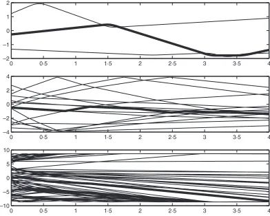
Figure 7 shows trajectories computed with the backward Euler method with the same step-length
∆t =1/k. This method has the shortcoming that particles tend to lose energy when they collide. This can already be observed forn=3 (by comparison with the previous figure) but worsens asnincreases. Forn =75, the particles quickly have very little energy and stick to the walls when they collide there. This could be improved by decreasing the step-length but the backward Euler method is already much more expensive than the symplectic Euler and could only be practical if a much longer time step were possible. Moreover, we believe that with the scaling∆t =γk, trajectories will become progressively worse with increasingnfor anyγ >0.
In Fig. 8, we show trajectories computed with the forward Euler with∆t =0·0039/k. The forward Euler has a strong tendency to add energy to the system at every collision. To obtain a comparable performance with symplectic Euler for smalln, it is necessary to take a vastly smaller step. Even with this smaller step, for largen the energy of the solution computed with forward Euler grows rapidly in time. We conjecture that if∆t =γ /∆t, for someγ >0, then the trajectory of the tracer particle will diverge as a stochastic process asn → ∞.
[image:17.595.222.416.121.301.2]0 0·5 1 1·5 2 2·5 3 3·5 4 –2
–1 0 1 2
0 0·5 1 1·5 2 2·5 3 3·5 4
–4 –2 0 2 4
0 0·5 1 1·5 2 2·5 3 3·5 4
–10 –5 0 5 10
FIG. 7. Trajectories computed with the backward Euler method with∆t = 1/k. Plots are of particle position versus time for
n=3,15,75,k=n2.
0 0·5 1 1·5 2 2·5 3 3·5 4
–2 –1 0 1 2
0 0·5 1 1·5 2 2·5 3 3·5 4
–4 –2 0 2 4
0 0·5 1 1·5 2 2·5 3 3·5 4
–10 –5 0 5 10
FIG. 8. Trajectories computed with the forward Euler method with∆t =0·0039/k. Plots are of particle position versus time for
n=3,15,75,k=n2.
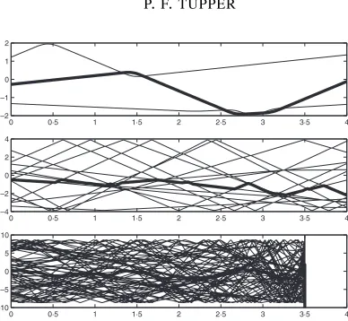
With a step-length of∆t =0·00028/k, whenn =75, overflow occurs neart =3·5 due to increasing energy.
Figure 10 shows trajectories computed with the projected symplectic Euler method with∆t=1/k. In this case, it is difficult to see any major difference between this computation and that with the regular symplectic Euler method. However, since the projected symplectic Euler method is more costly, the method would not be practical unless a longer step-length could be used than that used with the symplectic Euler.
[image:18.595.221.417.143.300.2] [image:18.595.222.416.345.505.2]0 0·5 1 1·5 2 2·5 3 3·5 4 –2
–1 0 1 2
0 0·5 1 1·5 2 2·5 3 3·5 4
–4 –2 0 2 4
0 0·5 1 1·5 2 2·5 3 3·5 4
–10 –5 0 5 10
FIG. 9. Trajectories computed with RK4 with∆t = 0·00028/k. Plots are of particle position versus time forn = 3,15,75,
k=n2.
0 0·5 1 1·5 2 2·5 3 3·5 4
–2 –1 0 1 2
0 0·5 1 1·5 2 2·5 3 3·5 4
–4 –2 0 2 4
0 0·5 1 1·5 2 2·5 3 3·5 4
–10 –5 0 5 10
FIG. 10. Trajectories computed with the projected symplectic Euler method with∆t=1/k. Plots are of particle position versus time forn=3,15,75,k=n2.
n =75, the net results of this non-local behaviour is that only a few particles have the vast majority of the energy in the system at any time.
6.3 Limiting statistics
[image:19.595.223.417.121.300.2]Clearly, none of the forward Euler, backward Euler or the RK4 methods will capture long-term statistics properly. Accordingly, for our experimental investigation of the preservation of statistical limits, we only consider the symplectic Euler method and its projected version. In the following, we will use the Gaussian distribution for the initial velocities.
Figure 12 showsC−Cn,k,∆t, withCn,k,∆t computed by the symplectic Euler method with∆t =
[image:19.595.222.415.339.499.2]0 0·5 1 1·5 2 2·5 3 3·5 4 –2
–1 0 1 2
0 0·5 1 1·5 2 2·5 3 3·5 4
–4 –2 0 2 4
0 0·5 1 1·5 2 2·5 3 3·5 4
–10 –5 0 5 10
FIG. 11. Trajectories computed with the projected symplectic Euler method with∆t =1·25/k. Plots are of particle position versus time forn=3,15,75,k=n2.
0 0·2 0·4 0·6 0·8 1 1·2 1·4 1·6 1·8 2
–0·1 –0·05 0 0·05 0·1 0·15 0·2 0·25 0·3 0·35 0·4
∆
t
n=3
n=15
n=75
C
(
t
)
– C
n,k, t
(
t
)
FIG. 12. Symplectic Euler method.C(t)−Cn,k,∆t(t)fort∈ [0,2], with∆t=1/k, andk=n2. The standard deviation of the
error on the curves never exceeds 0·002.
to explore. Since with the∆t ∼1/kscaling we are not resolving fine details of the collisions, we are not computing trajectories accurately in this limit.
We perform the same numerical experiment with the projected symplectic Euler method. Figure 13 showsC −Cn,k,∆t computed by this method. As before,∆t = 1/k,k = n2, andn =3,15,75.
Comparison with Fig. 12 shows that, forn =3,15, the method computes similar covariance functions to those of the non-projected method. However, forn =75, the covariance function appears different. It is difficult to ascertain from this plot whether convergence will occur asn → ∞with this step-length,
∆t = 1/k. In either case, the covariance function is not converging to C as rapidly as the regular symplectic Euler method converges, thus we know that the projection has some effect on the statistics.
0 0·2 0·4 0·6 0·8 1 1·2 1·4 1·6 1·8 2 –0·1
–0·05 0 0·05 0·1 0·15 0·2 0·25 0·3 0·35 0·4
C
(
t
)
Cn,k
,∆
t
(
t
)
t
n=3
n=15
n=75
FIG. 13. Projected symplectic Euler method.C(t)−Cn,k,∆t(t)fort∈ [0,2]withk=n2and∆t=1/k. The standard deviation
of the error on the curves never exceeds 0·005.
0 0·2 0·4 0·6 0·8 1 1·2 1·4 1·6 1·8 2
–0·8 –0·6 –0·4 –0·2 0 0·2 0·4
C
(
t
) –
Cn,k,
∆
t
(
t
)
t
n=3
n=15
n=75
FIG. 14. Projected symplectic Euler method.C(t)−Cn,k,∆t(t)fort ∈ [0,2]withk =n2and∆t = 1·25/k. The standard
deviation of the error on the curves never exceeds 0·005.
function is clearly not converging toC asn → ∞. These observations correspond with what we have previously observed in individual trajectories.
Acknowledgements
This work was done while the author was supported by the Thomas V. Jones Stanford Graduate Fellowship. The author would like to thank Andrew Stuart for helpful discussions. Special thanks go to Jason Swanson for pointing out a serious error in an earlier draft of this manuscript.
REFERENCES
BILLINGSLEY, P. (1999)Convergence of Probability Measures,2nd edn. New York: Wiley.
CANO, B., STUART, A. M., S ¨ULI, E. & WARREN, J. O. (2001) Stiff oscillatory systems, delta jumps and white noise.Found. Comput. Math.,1, 69–99.
DEUFLHARD, P., HERMANS, J., LEIMKUHLER, B., MARK, A. E., REICH, S. & SKEEL, R. D. (1999)
Computational Molecular Dynamics: Challenges, Methods, Ideas.Lecture Notes in Computational Science and Engineering. Berlin: Springer.
D ¨URR, D., GOLDSTEIN, S. & LEBOWITZ, J. L. (1980/81) A mechanical model of Brownian motion.Comm. Math. Phys.,78, 507–530.
DURRETT, R. (1996)Probability: Theory and Examples,2nd edn. Belmont, CA: Duxbury Press.
DVORETZKY, A. (1977) Asymptotic normality of sums of dependent random vectors. Multivariate Analysis–IV.
(P. R. Krishnaiah, ed.). Amsterdam: North Holland, pp. 23–34.
FORD, G. W. & KAC, M. (1987) On the quantum Langevin equation.J. Stat. Phys.,46, 803–810.
HAIRER, E., LUBICH, C. & WANNER, G. (2002)Geometric Numerical Integration: Structure-Preserving
Algo-rithms for Ordinary Differential Equations. Berlin: Springer.
HAIRER, E., NØRSETT, S. P. & WANNER, G. (1987)Solving Ordinary Differential Equations I: Nonstiff Problems.
Berlin: Springer.
HALD, O. H. & KUPFERMAN, R. (2002) Asymptotic and numerical analyses for models of heat baths.J. Stat. Phys.,106, 1121–1184.
HARRIS, T. E. (1965) Diffusion with ‘collisions’ between particles.J. Appl. Prob.,2, 323–338.
HOLLEY, R. (1971) The motion of a heavy particle in an infinite one dimensional gas of hard spheres.ZWVG,17,
181–219.
HUISINGA, W., SCHUTTE¨ , C. & STUART, A. M. (2003) Extracting macroscopic stochastic dynamics: model
problems.Comm. Pure Appl. Math.,56, 234–269.
KUPFERMAN, R., STUART, A. M., TERRY, J. R. & TUPPER, P. F. (2002) Long-term behaviour of large
mechanical systems with random initial data.Stoch. Dyn.,2, 533–562.
M ¨URMANN, M. G. (1973) A semi-Markovian model for the Brownian motion.S´eminar de Probabilit´e, VII, Lecture
Notes in Math., Vol 321. Springer, pp. 248–272.
PAOLI, L. & SCHATZMAN, M. (1993) Vibrations avec contraintes unilat´erales et perte d‘´energie aux impacts, en dimension finie.C. R. Acad. Sci. Paris S´er. I Math.,317, 97–101.
REISS, R.-D. (1989) Approximate Distributions of Order Statistics, Springer Series in Statistics. New York: Springer.
SIGURGEIRSSON, H. & STUART, A. M. (2001) Statistics from computations. Foundations of Computational
Mathematics (Oxford 1999), London Mathematical Society Lecture Note Series 284. Cambridge: Cambridge University Press, pp. 323–344.
SPITZER, F. (1968/1969) Uniform motion with elastic collision of an infinite particle system.J. Math. Mech.,18,
973–989.
STUART, A. M. & WARREN, J. O. (1999) Analysis and experiments for a computational model of a heat bath.J.
Stat. Phys.,97, 687–723.
TURAEV, D. & ROM-KEDAR, V. (1998) Elliptic islands appearing in near-ergodic flows.Nonlinearity,11, 575–
600.
Appendix A.
Recall the definition ofNnfrom (3.9). We need to establish the following result: For anyt1,t2, . . . ,td∈ [0,T], the random vector
converges in distribution to a Gaussian random vector with covariance matrixΣi j =C(ti −tj). Here,
C(t)is as defined in (2.5).
For our later convenience we define
Ft(x1,x2):=P{yj(0)x1,yj(t)x2}. (A1)
Since for each j the processyjis stationary, this implies
P{yj(t1)x1,yj(t2)x2} = Ft2−t1(x1,x2) for anyt1,t2∈ [0,T].
We apply a Central Limit Theorem of Dvoretzky (1977, Theorem 1). The result holds for certain dependent random vector arrays, but we will only need it for the independent case.
THEOREMA.1 (From Dvoretzky, 1977). For eachn, let Xn,i, 1 i n be independent random
column vectors inRdwithEXn,i =0. LetΣ be ad×dmatrix. For a vectorX, denote its norm by|X|
and its transpose byXT. For an eventA, let
E(X;A):=E(X1A).
Suppose
1. limn→∞
n
i=1EXn,iXnT,i =Σ,
2. for all >0, limn→∞
n
i=1E(|Xn,i|2; |Xn,i|> )=0.
ThenSn=Xn,1+ · · · +Xn,n⇒N(0,Σ)asn → ∞.
In our case,SnandXn,i are vectors of lengthd withSn,j = Nn,j andXn,i,j =n−1/2νn,i,j, where
Nn,j andνn,i,j are defined in (3.9) and (3.8) respectively. We proceed to check the hypotheses of the
CLT.
First note thatEn−1/2νn,i,j =0 for eachn,i,j. Furthermore, with some algebra and the fact that
E[1yi(tj)n−1/2xj] =(1+n
−1/2 xj)/2,
we obtain
n
i=1
E[(n−1/2νn,i,j)(n−1/2νn,i,k)]
=n−1
n
i=1
[−(1+n−1/2xj)(1+n−1/2xk)+4P{yi(tj)n−1/2xj,yj(tk)n−1/2xk}] =4Ftk−tj(n−
1/2
xj,n−1/2xk)−(1+n−1/2xj)(1+n−1/2xk)
where Ft is defined in (A1). It can be shown that Ft is continuous at(0,0)for all t ∈ [0,T], (for
example, by showing that Ft is Lipschitz in each variable there.) Hence the above quantity converges
In order to verify the final condition of the CLT theorem, observe that|νn,i,j|2 for alln,i,j, so n
i=1
E |(n−1/2νn,i,j)(n−1/2νn,i,k)|; d
l=1
|n−1/2νn,i,l|>
= n
i=1
n−1E |νn,i,j||νn,i,k|; d
l=1
|νn,i,l|>n1/2
E[4;2d >n1/2] =4P{2d >n1/2}
which converges to zero as required.
LEMMAA.2 We have
4Ft(0,0)−1=C(t).
Proof. We can rewriteFtas
Ft(z1,z2)=E[1qz11G(q+t p)z2] = 1 2 ∞ −∞ 1 −1
1qz11G(q+pt)z2dq f(p)dp. So
4Ft(0,0)−1=2
∞
−∞
1
−1
1q01G(q+pt)0dq f(p)dp−1=4
∞
−∞ ˜
H(pt)f(p)dp−1 where we have defined
˜
H(z):= 1 2
1
−1
1q01G(q+z)0dq.
In order to obtain a more explicit expression forH˜, we first observe that it will be periodic with a period of 4. Then some lengthy but straightforward calculations will show that
˜
H(z)=
(1−z)/2, 0z1,
0, 1z2,
(z−2)/2, 2z3,
1/2, 3z4.
We can take advantage of the fact that f is symmetric about 0: 4Ft(0,0)−1=4
∞
−∞ ˜
H(pt)(f(p)+ f(−p))/2 dp−1
=2
∞
−∞( ˜
H(pt)+ ˜H(−pt))f(p)dp−1
=
∞
−∞[2( ˜
H(pt)+ ˜H(−pt))−1]f(p)dp The expression in the square brackets happens to equalHof equation (2.4). So
4Ft(0,0)−1=
∞
−∞H(pt)f(p)dp=C(t)