Improving Compositional Verification of State based Models by Reducing Modular Unbalance

Improving Compositional Verification of State-based Models

by Reducing Modular Unbalance

Mauricio Varea

[email protected] [email protected]

Michael Leuschel

[email protected]

Bashir M. Al-Hashimi

Department of Electronics and Computer Science

University of Southampton, SO17 1BJ, UK

Abstract

Compositional Verification is a viable way to tackle the state explosion problem. However, the decomposition of a system into smaller parts is not a trivial problem, and dividing the specification into modules can be regarded as one of the main issues that concerns a compositional approach. This paper concentrates on the application of compositional verification to state-based models, in order to reduce the number of nodes assigned to memory, thus avoiding state explosion and speeding up the verification. Furthermore, we investigate and propose an estimation method that improves the compositional verification pro-cess in modular designs, such that the amount of memory required by the process is minimised. This method has been applied to a real-life embedded system, producing meaningful results without the need of data abstraction.

1

Introduction

In the design of large embedded systems, the designer of-ten faces a trade-off as to which validation technique to use in order guarantee that the final implementation will meet the specification. On the one hand, formal veri-fication techniques [4] aim to mathematically prove the correctness of a specification, but suffer from state explo-sion. On the other, simulation [5], testing [1], and refine-ment [2] can cope with larger specifications, but they do not cover the entire state space. The key aspect here is that simulation and testing are feasible for large models because they do not attempt to validate the entire specifi-cation at once. In other words, breaking down the spec-ification into smaller parts, called modules, would make the entire system specification formally verifiable, i.e., the model checker will give an answer as to whether or not the specification satisfies a temporal logic property, in a finite

time. This type of verification, known as modular or

com-positional verification, is a divide-and-conquer approach

that uses natural divisions in the specification in order to partition the structure and, therefore, reduce the number of states involved in the process.

Compositional verification was introduced in [8], aim-ing to reduce the complexity of large designs validation. Since then, the problem has been studied in several for-malisms [11, 15, 20], but not so often applied in computer-aided verification of real-world applications. Only in re-cent years there has been some increasing research effort towards developing tools and techniques to validate real-life embedded systems by compositional verification [22]. This includes, e.g., microprocessor architectures [16, 21], hardware protocols [23], multimedia SoC [28] and multi-agent systems [17].

The main contribution of this paper is an estimation of the complexity involved in the verification process when a modular approach is taken, which can be used to de-cide a priori which way to partition a state-based model. The estimator introduced in this paper is relevant for the design in terms of memory resources needed for the for-mal verification process. To the best of our knowledge, such estimator has not been developed in previous work. The concepts introduced in this paper are also applied to a real-world embedded system specification through a control/data-flow unbiased internal design representation, the Dual Flow Net (DFN) model [29, 30].

2

Compositional Verification

It is known that a small increment in the size of the model structure

M

, will result in a several-order-of-magnitude bigger state space to be explored [14]. Indeed, the ver-ification complexity, i.e., cost of applying formal verifi-cation to a system description in terms of memory re-sources, has been proved to be PSPACE-complete [18, 19]. Therefore, by decomposing

M

into n modules

{

M1

,

M2

, . . . ,

M

n}, in such a way that the parallel

com-position of all these modules

M1

k

M2

· · · k

M

nis

equiv-alent to the original structure

M

, it is possible to signifi-cantly reduce the number of states searched by the model checker, because the complexity is reduced. However, a model checker often uses some heuristic in order to avoid redundancy of larger state spaces and, by exploiting BDD’s features, also reduces the amount of BDD nodes allocated in memory. This means that a large number of very small modules

M

i does not necessarily lead to the

most efficient way to perform model checking, since they would not share any path in the verification process. In fact, there is a trade-off between having a vast number of small modules, which can have quite a substantial re-dundancy factor, and having only a few modules that are larger in size, which takes more memory resources due to the exponential rate of increase in the verification com-plexity.

Mathematically, the compositional verification of a structure

M

that has been constructed by the parallel com-position (i.e.,k) of modules

M

i, is formulated as:

M1

ϕ1

M2

ϕ2 · · ·

M

nϕn

f(ϕ1, . . . ,ϕ_n) =⇒ ϕ

M1

k

M2

· · · k

M

nϕ

which means that proving that each module

M

i,

∀1₆i₆n, satisfies the temporal logic formula ϕi, and

also proving that each formulaϕi is related to the

prop-ertyϕ(through a logical function f ), the conclusion that the entire system

M

satisfies the propertyϕcan be drawn. A key issue in compositional verification is the

assume-guarantee paradigm [24, 27], which bases its reasoning

in separating a system in two parts: the module

M

0_and

the environment

M

00_{. Guarantees}

G

iare properties of

M

0

which are verified assuming that

M

00 satisfies some as-sumptions

A

j. By appropriately combining a set of

as-sumptions

A

and a set of guarantees

G

, it is possible to infer the correctness of the entire system

M

without actu-ally building the global state-transition graph.

Let

M

0_{be any module of the system, and}

M

00_its

envi-ronment. This is,

M

=

M

0_k

M

00_{. The assume-guarantee}

paradigm states that:

M

00

A

A

k

M

0

G

M

00_k

T

Gϕ

M

ϕ

Where

T

Gis the “tableau of the property

G

”, as in [20].

3

Motivational Example

Assume that a ten-stage pipeline system needs to be for-mally verified. The property to be verified is simply that some data put at the beginning of the pipeline will prop-agate and eventually reach the end. The minimum unit of functionality of the system is each stage itself, but we will suppose that the system can only be partitioned into three separate modules, which will be assigned to three different hardware resources.

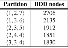
Partition BDD nodes h1,2,7i 2706

h1,3,6i 2135

h2,3,5i 1912

h2,4,4i 1851

[image:2.612.384.494.305.383.2]

h3,3,4i 1830

Table 1: Sizes of BDD trees for a ten-stage pipeline

Table 1 shows that different ways of partitioning this pipeline, i.e., grouping these pipeline stages, leads to dif-ferent complexities in terms of BDD nodes allocated to memory. The notationhx,y,ziindicates the size of each partition, where x+y+z is the total size of of the

sys-tem. This variety of partitioning schema raises the vexed question of how to identify which partitions would lead to better results in compositional verification.

4

The Estimation Method

Intuitively, a four-module system which has a partition

P=h4,4,4,4iis more balanced than the same system us-ing other partitionP0=h1,9,4,2i, where the elements in the tuple indicates the number of elementary units (tran-sitions t ∈T ) in each module. More formally,

Defini-tion 1 defines the modular unbalance of a Kripke struc-ture which has been partitioned under a partition scheme

P.

Definition 1 The modular unbalance of a Kripke

struc-ture

M

=

M1

k

M2

· · · k

M

nis given by:

σ=

s

1

n−1

n

∑

i=1

where ¯m is the statistical mean (average) of the sizes of

the modules, i.e., m=m/n.

It is clear from (1) that the unbalance is defined as the

standard deviation of the size of each module w.r.t. the

average size m=m/n. This can be seen as making

bal-ance analogue to volatility, since standard deviation is one of the most common ways to assess the volatility of a dis-crete variable. Thus, σ→0 corresponds to a very bal-anced system while σ→∞ is in accordance to an ex-tremely unbalanced system. A system withσ=0 will be called perfectly balanced, and a system with the greatest

σpossible will be called perfectly unbalanced. We make then the following proposition.

Conjecture 1 Among all possible partitions of a system

M

, the one which minimisesσwill also minimise the

ver-ification complexity.

The intuition, again, would serve to describe the fea-ture described in Proposition 1. Suppose a system

M

, which has a partition scheme P, which is perfectly bal-anced. Then, changingPintoP0implies that at least one transition t∈T has to be removed from a module

M

iand

added into other module

M

j. This will lead to a

decre-ment in the complexity verifying

M

iand an increment in

the complexity verifying

M

j. Since the exponential nature

of BDD’s state space, it is more likely that the improve-ment due to the reduction of

M

iis less than the worsening

caused by the expansion of

M

j. Therefore, the overall

in-creasing of the verification complexity is accompanied by an increase ofσ, and vice versa.

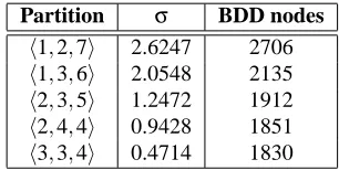
Partition σ BDD nodes h1,2,7i 2.6247 2706

h1,3,6i 2.0548 2135

h2,3,5i 1.2472 1912

h2,4,4i 0.9428 1851

[image:3.612.331.548.281.414.2]

h3,3,4i 0.4714 1830

Table 2: Estimating the pipeline complexity

Coming back to the example presented in Section 3, Table 2 show that the more balance, i.e.σ→0, the less number of BDD nodes allocated in memory. This leads to an improvement of, in this case, 32% in the resources allocated to the BDD tree, although in all cases the veri-fication is performed over the same system with the same properties. Therefore, this has provided an answer to the question raised earlier and we believe that it is important to includeσas an estimation method to guide the parti-tion of a system which will be further verified by compo-sitional methods.

However, the size of each module is not the only issue that concerns the verification complexity. The coupling among modules is equally important for verification pur-poses, and being able to find the proper

T

_Gdetermines the satisfaction of the results. Due to the internal behaviour of the model checker, which unfolds cycles to perform the verification, all results hitherto presented assume that modules are set to be free of cycles. Otherwise, well bal-anced partitions may have bigger unfolded structure than others less balanced and, thus, more complex BDD trees. This is illustrated in Figure 1, where the solid line indi-cates the results shown in Table 2 while the dashed line represents the same pipeline constructed with a cycle in the specifications. It can be observed that, between two partitionsPandP0, withσ<σ0, the complexity ofPwill be less than the one fromP0, only in the acyclic case.

acyclic cyclic

1800 1900 2000 2100 2200 2300 2400 2500 2600 2700 2800

0 0.5 1 1.5 2 2.5 3

BDD nodes

Standard Deviation

Figure 1: Cyclic and acyclic complexity

An automatic approach to the compositional verifica-tion problem would search through a space of possible modular partitions of the DFN model, in order to obtain a the one with minimumσ. Although this approach goes beyond the scope of this paper, we will give an insight of the theoretical limits of our methodology.

It has been proven in [13] that the number of distinct partitions for a modular design is:

#P(m)≈

exp

πq2m 3

4m√3 (2)

where m=|T|is the number of transitions in the model. However, we argue that not all Pi, 16i6#P(m), are

[image:3.612.109.262.469.546.2]

5

A Real-life Example

This section applies the estimation method proposed to a real-life embedded system, i.e., the Ethernet network’s coprocessor, in order to show that the compositional veri-fication of such systems also benefits from the improve-ments introduced by the method. The Ethernet copro-cessor is a chip advocated to transmitting and receiving data frames over a communication channel by means of the CSMA/CD protocol, which is defined in the IEEE 802.3 standard [3]. In order to model the coprocessor, a control/data-flow unbiased internal design representa-tion has been used, and the formal verificarepresenta-tion process has been carried out with the use of the Cadence SMV tool [6]. The platform used was a Sparc Sun-Ultra 10 / 440 MHz with 512 Mb RAM running Solaris 8.

5.1

The Model: Dual Flow Nets

The Dual Flow Net (DFN) model [29, 30] is an exten-sion to the Petri net (PN) model which introduces a com-bined control/data-flow analysis of systems. This model utilises a set of vertices (P) to represent the state/storage elements in the system, another set of vertices (T ) to cap-ture the control flow, and an additional set (Q), not present in PNs, for capturing the transformational elements in the system. A set of arcs F⊆(P×T)∪(T×P)∪(P×

Q)∪(Q×P)∪(T×Q)∪(Q×T)and a weight function

W : F7→Z\∅ define the model structure, as well as a

marking function defined in the domain of the complex numbers (µ : P7→C/ _{) characterise its behaviour. In}

addi-tion, there also exist a guard function G : T 7→]∪ {>}, where] is a finite set of symbols used for comparison, and an offset function H : Q7→Z, which complements the functionality of the model by allowing some arithmetical and logical functions to take place.

Since the DFN model has an enhanced structure, i.e., it contains an additional set (Q) which explicitly captures data activity, this model can be used to verify embedded systems [31]. If a model such as PN was used instead, only the control part would have been verified. Thus, the underlying PN that is visualised when all transforma-tional elements are removed from a DFN model, behaves with the same enabling and firing rule of a classical PN. However, on each transition firing a number of operations take place in the data domain. Further discussion on this model, as well as a formal definition of its principles, the motivation and some introductory examples, can be found in [29].

5.2

An Ethernet network coprocessor

The Ethernet network coprocessor, as studied in [12] and [26], is a highly structured protocol. This makes it very suitable for a benchmark of real-life complexity, mainly if compositional methods are going to be applied. There have been a few attempts to perform formal ver-ification of this coprocessor. For example, one of the earliest work on the verification of the Ethernet protocol was presented in [25]. This approach has used the SMV tool1to verify both the asynchronous and the synchronous model [32] of the Ethernet. Later, another approach di-rectly implemented in C has presented the formal verifi-cation of some liveness properties using approximations to cope with the state explosion [10].

The operation of the coprocessor is ruled by the exe-cution unit, exec unit, which sends the starting memory address to the transmit unit (composed of a frame pack-ager xmit frame, a direct memory access (DMA) unit

dma xmit), and a serial transmitterxmitbit) and then en-ables the DMA unit to operate straight into memory.

Thedma xmit unit directly reads from the successive memory locations in order to obtain destination address, data length, and the actual data, which are then sent to the

xmit frameunit. There are two modes of operation in the

dma xmit unit: dma xmit normal and dma xmit cancel, so that this unit normally stays in the first mode but, if a failure occurs in the transmission toxmit frame, the DMA unit switches to an alternative mode that sets up the envi-ronment to restart the transmission process.

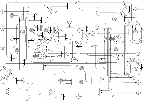
The specification presented above has been captured by the DFN model introduced in Section 5.1. Figure 2 shows the complete model consisting of 49 places, 36 transitions and 12 hulls. As commented in Section 2, a model with 36 transitions would imply that there are 19,370 ways to group these transitions into different modules. However, by identifying threads of executions with no cycles in it (e.g.{t7,t34,t8}), the number of practically implementable

modules is reduced from 36 to just 8, which means that #P(m)is also dramatically reduced (to 26). This mod-ules have been denoted by:

M1

,

M2

, . . . ,

M8

. As a matter of notational convenience, the one place that precedes a module

M

i has been labelled pi,∀1<i<8, and

high-lighted in Figure 2. The importance of identifying these places lies on the fact that any token coming into the area of

M

i, has to go through pi. That is the basis for applying

modularisation of such DFN models.

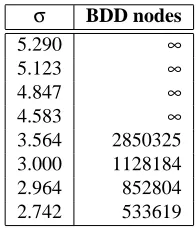
Different alternatives for the modularisation are shown in Table 3. The∞symbol indicates that state explosion has occurred and the model checker was unable to find a solution in a reasonable amount of time. Further results

σ BDD nodes

5.290 ∞

5.123 ∞

4.847 ∞

4.583 ∞

3.564 2850325

3.000 1128184

2.964 852804

[image:5.612.137.235.73.187.2]

2.742 533619

Table 3: Balance vs. complexity

presented in this section, are based on the row which has the lessσ.

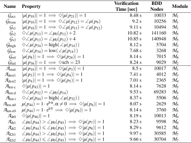
In order to prove the correctness of the Ethernet copro-cessor by compositional verification, 22 temporal formu-las have been used. Table 4 shows the verification results for each property, where the first 9 are guarantees

G

i, and

the remaining 13 are assumptions

A

j. It can be observed,

from the fourth column, the complexity of the verifica-tion measured by the amount of BDD nodes allocated into memory.

The behaviour of the model is captured through the guarantee set of properties. For example, when atxstart

signal is sent to the DMA unit, this will request access to the CPU (c.f.

Gacc

). Then, the system reads from suc-cessive memory locations (c.f.

Gs1

,

Gs2

and

Gs3

), starting fromtxaddress_[16](c.f.

Gfrom

). At this point, the Ethernet

coprocessor is ready to transmitBdata_[16]toxmit frame,

but this is a 8 bit unit. So, we formulate

Ghigh

and

Glow

in order to prove that bothBdata_[15..8]andBdata[7..0]are

transfered to such unit.

However, it is not sufficient to prove these nine

G

i. In

order to complete the proof, we need to assure liveness and declare the order and dependences of the modules mentioned above. By means of

A

j we prove that each

module will eventually call another module (i.e., the DFN model is live) and we guide the control flow according to some intermediate data values placed in p44 and p45.

Therefore, the correctness of this DFN model has been proven within 190.45 seconds –as opposed to the state explosion suffered if we were to apply the methodology without any modularity.

6

Conclusions

We have examined the way to break down a complex specification in compositional verification, such that the amount of memory resources used is reduced. For this, we have proposed an estimation method that tackles the modular unbalance of a structure and aims to reduce the

complexity by careful selection of the way the system is partitioned. It should be noted that the method and con-clusions showed in this paper are not limited to any model in particular and can be applied to many internal design representations that allows modular decomposition. How-ever, the method is slightly restricted by the fact that sys-tems with uneven communication needs (as opposed to the the pipeline example) or systems which include cycles in their behaviour may respond in a different way and, therefore, be optimised by a different partitioning scheme. Thus, although the proposed method might not be opti-mal, it provides a good indication to efficiently partition a structure in terms of verification time. In order to val-idate the estimation method, it has been tested by means of a real-life example, showing that it can be successfully applied to models of relatively large complexity.

References

[1] Miron Abramovici, Melvin A. Breuer, and Arthur D. Friedman. Digital Systems Testing and Testable Design. IEEE Computer Society Press, MD 20910, USA, 1990.

[2] Jean-Raymond Abrial. The B-Book. Cambridge Press, 1996.

[3] ANSI/IEEE. Information Processing Systems – Local Area Networks – Part 3: Carrier Sense Multiple Access with col-ision Detection (CSMA/CD) access method and physical Layer Specifications. The IEEE, Inc., N.Y., October 1991.

[4] B. B´erard, M. Bidoit, A. Finkel, F. Laroussinie, A. Petit, L. Petrucci, Ph. Schnoebelen, and P. McKenzie. Systems and Software Verification: Model-Checking Techniques and Tools. Springer-Verlag, Berlin, Germany, 2001.

[5] Michael L. Bushnell and Vishwani D. Agrawal. Essen-tials of Electronic Testing for Digital, Memory and Mixed-Signal VLSI Circuits. Kluwer Academic Publishers, Dor-drecht, The Netherlands, 2001.

[6] Cadence. The SMV Model Checker.

http://www-cad.eecs.berkeley.edu/∼kenmcmil/smv/,

2001.

[7] Proceedings of the 7thInternational Conference on

Com-puter Aided Verification, volume 939 of Lecture Notes in Computer Science, Li`ege, Belgium, 3-5 July 1995. Springer-Verlag.

[8] Edmund M. Clarke, David E. Long, and Kenneth L. McMillan. Compositional Model Checking. In Proceed-ings of the 4thIEEE Symposium on Logic in Computer Sci-ence, pages 353–362, 1989.

[9] CMU. The SMV System.

http://www.cs.cmu.edu/∼modelcheck/smv.html, 1997.

Name Property Verification Time [sec]

BDD

Nodes Module

Gacc

|µ(p10)|=1 =⇒ 3|µ(p21)|=1 8.48 s 10033

M1

Gfrom

|µ(p10)|=1 =⇒ 3∠µ(p12) =∠µ(p9) 9.2 s 10256

M1

Gs1

|µ(p10)|=1 =⇒ 3∠µ(p13) =∠µ(p12) 9.11 s 10494

M1

Gs2

3∠µ(p13) =∠µ0(p12) +2 10.82 s 141160

M5

Gs3

3∠µ(p13) =∠µ0(p12) +4 10.85 s 140948

M5

Ghigh

3∠µ(p34) =high(∠µ(p14) ) 8.12 s 5704

M3

Glow

3∠µ(p34) =low(∠µ(p14) ) 7.68 s 3268

M4

Grel

|µ(p8)|=1 =⇒ 3|µ(p26)|=1 8.14 s 7015

M8

Gfail

|µ(p36)|=1 =⇒ 3sch=23 8.24 s 9029

M2

Astart

|µ(p10)|=1 =⇒ 3|µ(p3)|=1 8.5 s 10017

M1

Adest1

|µ(p3)|=1 =⇒ 3|µ(p4)|=1 7.41 s 4012

M3

Adest2

|µ(p4)|=1 =⇒ 3|µ(p5)|=1 7.01 s 2365

M4

Alen-c

3|µ(p43)|=1 8.14 s 7628

M5

Alen-d

3∠µ(p32) =∠µ0(p14) 9.53 s 69283

M5

Alen-i

3∠µ(p44) =high(∠µ(p32) ) 8.37 s 5506

M5

Alen-n0

µ(p44) =1·ei·α,α6=0 =⇒ 3|µ(p6)|=1 8.07 s 2629

M5

Alen-e0

µ(p44) =1·ei·0 =⇒ 3|µ(p8)|=1 8.14 s 3760

M5

Adt0

3|µ(p46)|=1 8.19 s 10013

M6

[image:6.612.119.506.74.365.2]

Adt1

∠µ0(p44)>∠µ0(p45) =⇒ 3|µ(p7)|=1 8.23 s 9598

M6

Adt2

∠µ0(p44)6 ∠µ0(p45) =⇒ 3|µ(p8)|=1 8.29 s 9612

M6

Ad2t1

∠µ0(p44)>∠µ0(p45) =⇒ 3|µ(p6)|=1 9.97 s 30585

M7

Ad2t2

∠µ0(p44)6 ∠µ0(p45) =⇒ 3|µ(p8)|=1 9.66 s 30704

M7

Table 4: Ethernet LTL properties

[11] Orna Grumberg and David E. Long. Model Checking and Modular Verification. ACM Transaction on Programming Languages and Systems, 16(3):843–871, 1994.

[12] Rajesh K. Gupta and Giovanni De Micheli. System Syn-thesis via Hardware-Software Co-Design. Technical Re-port CSL-TR-92-548, Stanford University, Computer Sys-tems Laboratory, 1992.

[13] G. H. Hardy and S. Ramanujan. Asymptotic Formulae in Combinatory Analysis. Proceedings of the London Math-ematical Society, 17:75–115, 1918.

[14] David Harel, Orna Kupferman, and Moshe Y. Vardi. On the Complexity of Verifying Concurrent Systems. Imperial College, 173:143–161, 2002.

[15] Thomas A. Henzinger and Rajeev Alur. Local Liveness for Compositional Modeling of Fair Reactive Systems. In CAV [7], pages 166–179.

[16] Ranjit Jhala and Kenneth L. McMillan. Microarchitecture Verification by Compositional Model Checking. In Pro-ceedings of the CAV’01, volume 2102 of Lecture Notes in Computer Science, pages 396–410, Paris, France, 18-22 July 2001. Springer-Verlag.

[17] Catholijn M. Jonker and Jan Treur. Compositional Ver-ification of Multi-Agent Systems: a Formal Analysis of Pro-activeness and Reactiveness. International Journal of Cooperative Information Systems, 11(1-2):51–91, 2002.

[18] D. Kozen and J. Tiuryn. Logics of Programs. In J. van Leeuwen, editor, Handbook of Theoretical Computer Sci-ence, pages 789–840. North Holland, Amsterdam, 1989.

[19] Orna Kupferman, Moshe Y. Vardi, and Pierre Wolper.

Module Checking. Information and Computation,

164(2):322–344, 2001.

[20] David E. Long. Model Checking, Abstraction, and Com-positional Verification. Ph.D. Thesis, Carnegie Mellon University, School of Computer Science, Pittsburgh, PA 15213-3891, USA, July 1993.

[21] Kenneth L. McMillan. Verification of an Implementation of Tomasulo’s Algorithm by Compositional Model Check-ing. In Proceedings of the CAV’98, volume 1427 of Lec-ture Notes in Computer Science, Vancouver, BC, Canada, 28 June - 2 July 1998. Springer-Verlag.

[22] Kenneth L. McMillan. A Methodology for Hardware Ver-ification using Compositional Model Checking. Science of Computer Programming, 37(1-3):279–309, 2000.

[23] Kenneth L. McMillan. Parameterized Verification of

the FLASH Cache Coherence Protocol by Compositional

Model Checking. In Proceedings of the CHARME’01,

p 26 t 20 p 18 p 17 p 30 t 15 p 16 p 31 t 28 p 31 p 29 p 30 p 25 t 24 t 37 p 35 p 38 p 36 p 33 t 32 t 10 q 36 t 10 t ’=’ / 35 t 11 t 2 p 8 p 7 p 28 t 24 p 14 t 13 p 14 p 34 p 9 p 10 p 1 p 1 t 1 q 2

t q2

47 p

3 t

33

p q4

5 t 6 t 11 p 4 p 5 p 7 t 8 t 43 p 4 t 12 p 44 p 3 p 18 t 21 t 8 q 9 t 2−8

2−8 28

32 p 3 q 34 t 41 p 12 q 15 t 39 p 19 p 5 q 6 q 2−8 49 p 6 p 12 t 20 t 22 t 23 t 16 t 46 p 13 t 42

p q7

48 p 40 p 17 t 45 p 11 q 9 q 23 p 21 p 22 p 27 t 26 p 27 p 19

t t29

[image:7.612.72.552.71.408.2]

25 +2 +1 ’0’ "Bhold" ’0’ "Brd" "cancel" ’>=’ ’=’ "Bholdak" −1 ’>=’ ’<’ ’<’

Figure 2: DFN model of the Ethernet coprocessor

[24] Jayadev Misra and K. Mani Chandy. Proofs of Networks of Processes. IEEE Transaction on Software Engineering, 7(4):417–426, July 1981.

[25] Vivek G. Naik and A. P. Sistla. Modeling and Verifica-tion of a Real Life Protocol Using Symbolic Model

Check-ing. In Proceedings of the 6thInternational Conference on

Computer Aided Verification (CAV), 1994.

[26] Sanjiv Narayan and Frank Vahid. Modeling with SpecCha-rts. Technical Report ICS-TR-90-20, University of Cali-fornia, Irvine, Department of Information and Computer Science, October 1992.

[27] Amir Pnueli. In Transition for Global to Modular Temporal Reasoning. In K. R. Apt, editor, Logics and Models of Concurrent Systems, volume 13 of NATO ASI series. Series F, Computer and System Sciences. Springer-Verlag, 1984. [28] Subir K. Roy, Hiroaki Iwashita, and Tsuneo Nakata.

For-mal Verification based on Assume and Guarantee Aproach - A Case Study. In Proceedings of the Asia and South Pa-cific Design Automation Conf. (ASP-DAC), pages 77–80, Yokohama, Japan, 25-28 January 2000.

[29] Mauricio Varea. Mixed control/data-flow

representa-tion for modelling and verificarepresenta-tion of embedded systems.

MPhil/PhD-Transfer Report, Department of Electronics and Computer Science, University of Southampton, SO17 1BJ, UK, March 2002.

[30] Mauricio Varea and Bashir M. Al-Hashimi. Dual Transi-tions Petri Net based Modelling Technique for Embedded Systems Specification. In Proceedings of the DATE’01, pages 566–71, Munich, Germany, 13-16 March 2001. ACM/IEEE.

[31] Mauricio Varea, Bashir M. Al-Hashimi, Luis A. Cort´es,

Petru Eles, and Zebo Peng. Symbolic Model

Check-ing of Dual Transition Petri Nets. In ProceedCheck-ings of the CODES’02, pages 43–48, Colorado, USA, 6-8 May 2002.