Distributed shared memory architectures and global performance state estimation

(1)

Global Performance State Estimation

A Thesis

Submitted to the Office of Graduate Studies

of

The University of Dublin

Trinity College

in Candidacy for the Degree of

Doctor of Philosophy

by

Michael Manzke

(2)

(3)

Declaration:

This thesis has not been submitted as an exercise for a degree at this or any other Uni-versity. Furthermore this thesis is entirely my own work and I agree that the Library may lend or copy the thesis upon request. This permission covers only single copies made for study purposes, subject to normal conditions of acknowledgement.

(4)

Invasive and non-invasive methods may be applied to measure and analyse the perfor-mance of hardware Distributed Shared Memory (DSM) systems. This thesis presents novel solutions for both methods and discusses the architectural organisation of loosely and tightly coupled systems. The work begins with a discussion of the design and implementation of a non-invasive deep-trace instrument for high-speed interconnects and also deals with the analysis of the trace-data. Analysis results are used to tune interconnect simulations.

This thesis then presents an innovative invasive approach to estimate and predict the system-wide utilisation of computational resources in real-time. An algorithm that imple-ments a discrete minimum mean-square error filter is applied to fuse concurrent and se-quential observations of system event counts into a state-vector. Contemporary computer components and subsystems make these event counts available through hardware Perfor-mance Monitoring Counter (PMC) registers. The registers may be accessed by the system’s software quasi-concurrently but the number of registers in individual components is usually smaller than the number of events that can be monitored. This approach overcomes the problem by modelling individual PMC readings as vector random processes and recursively processes them one PMC set at a time into a common state-vector, thereby making larger PMC sets observable than would otherwise be possible.

(5)

My sincerest thanks and gratitude goes to Dr. Brian Coghlan and Prof. John Byrne. I thank Brian for taking me on as research assistant and postgraduate student on the SCI Europe project. At that time, I had spent a decade as an engineer in various positions in industry, subsequent to the completion of my engineering degree. Brian introduced me to many aspects of computer architecture and provided guidance for my PhD. He also gave me the freedom to pursue my own research interest. Prof. Byrne, who was at the time Head of Department, offered me the opportunity to prove myself as a lecturer. The income arising from this position allowed me the continue with my PhD. I could not have achieved this without them.

My children Denis, Rachel and Oscar and my wife Carol deserve a special mention here. I thank my children for coping with their parent’s very busy life style and Carol for looking after the family when I was not available. Carol is not only an outstanding researcher; she also enables me to pursue my academic career. I appreciate very much what Denis, Rachel, Oscar and Carol have done for me to make this possible and to Carol a special thanks for the many extra hours and weekends that I could dedicate to the completion of my PhD. I could not have done this without her support.

I would also like to thank my postgraduate students Ross Brennan, Eoin Creedon and Muiris Woulfe for all the support with the teaching, particularly the demonstrating and the marking of assignments.

The reviewers of my PhD-related publications deserve a thank you for their valuable feedback.

Furthermore I would like to thank the Head of Department Prof. Jane Grimson, the Head of School, Dr. David Abrahamson, and all my colleagues (there are too many to mention them all) for making our department such a nice and supportive environment. I should specifically mention the chief technician Tom Kearney. Tom and his group are an incredible help with my teaching and research activities.

(6)

Corpora-tion (Ireland, USA), Intel (Ireland), Motorola (USA). I would like to menCorpora-tion in particular Detlev Bock and Hilger Walter from Dow Chemical who introduced me to advanced process control and Kalman filtering during my time at Dow.

(7)

Abstract iv

Acknowledgments i

Table of Contents vi

List of Figures xi

List of Tables xii

Nomenclature xiv

List of Abbreviations xv

1 Introduction 23

1.1 Non-Invasive SCI Trace Data Acquisition . . . 23

1.2 Global Real-time Estimation of Incomplete Performance Measurements . . . 24

1.3 Special Purpose High Performance Graphics DSM Cluster . . . 24

1.4 Contributions . . . 25

1.4.1 Thesis Statement . . . 26

1.4.2 Directly Relevant Peer Reviewed Publications . . . 26

1.4.3 Indirectly Relevant Peer Reviewed Publications . . . 26

1.5 Thesis Organisation . . . 27

2 Motivation 29 2.1 Trace Data Acquisition and Analysis . . . 30

2.1.1 The SCI Non-Intrusive Deep Trace Instrument . . . 30

2.1.2 Tuning and Validation of SCI Network Models . . . 32

2.2 Global State Estimation of Hardware DSM Systems . . . 33

2.3 MMSE Filter Algorithm . . . 36

2.4 Distributed MMSE Filter Algorithm . . . 36

(8)

3 Background and Related Work 39

3.1 The Performance Analysis . . . 39

3.1.1 Performance Counter. . . 41

3.1.2 Multiplexed Performance Counter Readings . . . 41

3.1.3 Cluster wide PMC Collection . . . 41

3.2 Trace Data Acquisition and Analysis Related Work . . . 42

3.3 Kalman Filtering . . . 42

3.3.1 MMSE Filter Related Work . . . 43

3.4 Compute Cluster . . . 43

3.4.1 Interconnect Technologies . . . 43

3.4.2 Scalable Coherent Interface (SCI). . . 44

3.5 Special Purpose Graphics Cluster . . . 45

4 High Speed Interconnect Trace Data Acquisition and Analysis 47 4.1 SCI Trace Instrument Hardware . . . 47

4.1.1 Trace Probes . . . 48

4.1.2 Probe Adapter . . . 49

4.1.3 Trace Memory Boards . . . 50

4.1.4 Control Software . . . 50

4.2 SCI Trace Database . . . 51

4.2.1 SCI Cable-link Tables . . . 51

4.2.2 Blink Tables . . . 51

4.2.3 Trace Database Performance . . . 53

4.3 SCI Trace Data Presentation and Analysis . . . 55

4.3.1 Java Trace Database Server . . . 55

4.3.2 Java Packet Viewer Applet . . . 55

4.4 Tuning and Verification of Simulation Models . . . 57

4.4.1 SCI Simulation Model . . . 57

4.4.2 SCI Simulation Model Tuning . . . 59

4.5 Summary . . . 61

5 State Estimation of a Single Compute Node 62 5.1 The Estimation Algorithm. . . 62

5.1.1 The Filter . . . 63

5.1.2 PMC Process Models . . . 69

5.1.3 Integrated Gauss-Markov Process Model forn Counter Processes . . . 70

5.2 PMC Acquisition and Offline Analysis . . . 71

5.2.1 Acquisition of PMC readings . . . 72

5.2.2 Visual Inspection of sample PMC Readings and their Histograms . . . 73

(9)

5.2.4 Autocorrelation Calculation for Sampled PMC Readings . . . 73

5.2.5 Autocorrelation Calculation for Simulated PMC Readings . . . 75

5.2.6 Calculation of the Sampled PMC Readings’ Mean Autocorrelation . . 75

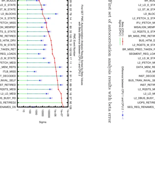
5.2.7 Calculation of the Simulated PMC Readings’ Mean Autocorrelation . 77 5.2.8 Estimation of β and σ2 for Sampled PMC Readings . . . 77

5.2.9 Estimation of β and σ2 for Simulated PMC Readings . . . 80

5.2.10 Visual Inspection of Histograms for Sampled PMC Readings . . . 80

5.2.11 Visual Inspection of Histograms for Simulated PMC Readings. . . 82

5.2.12 Autocorrelation Analysis Results . . . 82

5.3 One Performance Monitoring Counter (PMC) Set-at-a-Time . . . 86

5.4 Implementation of the Estimation Algorithm . . . 87

6 Optimisation and Re-evaluation of the Estimation Algorithm 95 6.1 Sparse Matrix Optimisation . . . 95

6.1.1 The Kalman Gain . . . 95

6.1.2 The A Posteriori State Estimate . . . 99

6.1.3 The A Posteriori Error Covariance . . . 102

6.1.4 The A Priori State Vector . . . 104

6.1.5 The A Priori Error Covariance Matrix . . . 105

6.2 Optimisation Analysis . . . 108

6.3 Uniprocessor Systems Evaluation . . . 116

6.3.1 Derived Performance Measurements . . . 118

6.4 SMP Systems Evaluation . . . 120

6.5 Distributed State Estimation . . . 122

7 Hardware DSM Testbeds 123 7.1 Loosely Coupled Distributed Shared Memory Testbed . . . 124

7.2 Tightly Coupled High Performance Graphics DSM Cluster . . . 126

7.2.1 Cluster Architecture . . . 127

7.2.2 Interconnect Technology . . . 130

7.2.3 Commodity and Custom-built GPU/FPGA Cluster Nodes. . . 131

8 Compute Cluster State Estimation Algorithm (C2_STATE) ₁₃₄ 8.1 The C2STATE Algorithm . . . 135

8.2 Shared Memory Clusters . . . 136

8.3 Work Loads . . . 141

9 Conclusions and Future Work 142 9.1 Performance Analysis . . . 142

(10)

9.2 Limitations and Future Work . . . 144

9.2.1 SCI Trace Acquisition and Analysis . . . 144

9.2.2 C2STATE Algorithm . . . 145

9.2.3 Interconnect Measurements . . . 145

9.2.4 Tightly Coupled Scalable Graphics Cluster . . . 146

9.2.5 Implementation of the C2STATE Algorithm on the Graphics Cluster . 146 9.2.6 Contributions . . . 146

A Appendix:PIII Performance Monitoring Counters (PMC) Description 147 B Appendix: PMC Offline Autocorrelation Analysis 157 B.1 PMC Offline Autocorrelation Analysis Procedure . . . 157

B.1.1 Histogram and Samples for real PMC Readings . . . 157

B.1.2 Histogram and Samples for Simulated Readings . . . 161

B.1.3 Histogram and Autocorrelation for Real PMC Readings . . . 163

B.1.4 Histogram and Autocorrelation for Simulated Readings . . . 166

B.1.5 Histogram of Real PMC Readings with superimposed Gaussian PDF . 168 B.1.6 Histogram of Simulated Readings with superimposed Gaussian PDF . 171 B.2 PIII PMC off-line autocorrelation analysis results. . . 173

Bibliography 196

(11)

2.1 Trace data flow overview . . . 31

2.2 Trace Data Acquisition and analysis framework . . . 33

2.3 Multiplexed sets of performance counter readings . . . 36

2.4 SMP Sample Time . . . 37

3.1 SMP Desktop Node with 2D SCI-PCI interface card. . . 45

4.1 SCI Deep Trace Instrument Front. . . 47

4.2 SCI Deep Trace Instrument Back . . . 47

4.3 Trace hardware overview including three possible trace targets . . . 48

4.4 Trace probe block diagram . . . 49

4.5 Probe adapter block diagram . . . 49

4.6 Trace memory board block diagram . . . 49

4.7 Trace instrument control GUI . . . 49

4.8 Trace instrument trigger and filter GUI . . . 50

4.9 Trace memory viewer. . . 50

4.10 Trace data flow from Blink into DB-table-files . . . 52

4.11 Packet trace database distribution . . . 54

4.12 Trace database relations . . . 55

4.13 Java Packet Viewer . . . 55

4.14 Trace system software . . . 56

4.15 SCI node OPNET model including PCI-bridge and Blink . . . 58

4.16 The points of measurement . . . 60

4.17 Probability density function . . . 60

4.18 Load definition . . . 60

4.19 Model output . . . 60

5.1 Histogram and samples for L2 LINES IN on CPU 1 . . . 63

5.2 Histogram and samples for L2 LINES IN on CPU 2 . . . 64

5.3 Discrete Kalman Filter Algorithm . . . 65

(12)

5.5 Integrated Gauss-Markov Block Diagram . . . 69

5.6 Histogram and samples for a simulated event . . . 73

5.7 Histogram and autocorrelation for L2 LINES IN on CPU 1 . . . 74

5.8 Histogram and autocorrelation for L2 LINES IN on CPU 2 . . . 74

5.9 Histogram and autocorrelation for a simulated event . . . 75

5.10 Autocorrelations and mean autocorrelation for L2 LINES IN on CPU 1 . . . 76

5.11 Autocorrelations and mean autocorrelation for L2 LINES IN on CPU 2 . . . 76

5.12 Autocorrelations and mean autocorrelation for simulation . . . 77

5.13 Autocorrelation Function . . . 78

5.14 Curve Fitted Autocorrelation for L2 LINES IN on CPU 1 . . . 79

5.15 Curve Fitted Autocorrelation for L2 LINES IN on CPU 2 . . . 79

5.16 Curve Fitted Autocorrelation for simulation . . . 80

5.17 Histogram of L2 LINES IN with superimposed Gaussian PDF for CPU 1 . . 81

5.18 Histogram of L2 LINES IN with superimposed Gaussian PDF for CPU 2 . . 81

5.19 Histogram of simulation with superimposed Gaussian PDF . . . 82

5.20 First set of autocorrelation analysis results with beta error . . . 83

5.21 First set of autocorrelation analysis results with sigma error . . . 83

5.22 Second set of autocorrelation analysis results with beta error . . . 84

5.23 Second set of autocorrelation analysis results with sigma error . . . 84

5.24 Third set of autocorrelation analysis results with beta error . . . 85

5.25 Third set of autocorrelation analysis results with sigma error . . . 85

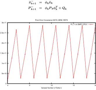
5.26 A Priori Error Covariance matrix element one of the major diagonal. . . 87

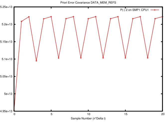
5.27 A Priori Error Covariance matrix element two of the major diagonal. . . 88

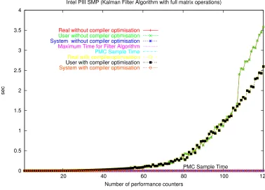
5.28 Full Kalman Operations on a Intel P4 . . . 92

5.29 Full Kalman Operations on a 2 way Intel PIII SMP . . . 92

5.30 Full Kalman Operations on a Intel PIII CompactPCI system . . . 93

5.31 Full Kalman Operations on a Intel P4 high resolution . . . 93

5.32 Full Kalman Operations on a 2 way Intel PIII SMP high resolution . . . 94

5.33 Full Kalman Operations on a Intel PIII CompactPCI system high resolution . 94 6.1 Sparse Kalman Operations on a Intel P4 . . . 110

6.2 Sparse Kalman Operations on a 2 way Intel PIII SMP . . . 110

6.3 Sparse Kalman Operations on a Intel PIII CompactPCI system . . . 111

6.4 Sparse Kalman Operations on a Intel P4 high resolution . . . 111

6.5 Sparse Kalman Operations on a 2 way Intel PIII SMP high resolution . . . . 112

6.6 Sparse Kalman Operations on a Intel PIII CompactPCI system high resolution112 6.7 Sparse Full Filter Operations in all Systems. . . 113

6.8 Sparse Full Filter Operations in all Systems high resolution . . . 113

(13)

6.10 Sample Time to User System Time Ratio in all Systems . . . 114

6.11 Sample Time to User System Time Ratio in all Systems high resolution . . . 115

6.12 Sample Time to User System Time Ratio in all Systems very high resolution 115 6.13 One-at-time Filter - two state variables. . . 116

6.14 One-at-time Filter - one state variable - short . . . 117

6.15 One-at-time Filter - one state variable . . . 117

6.16 Uniprocessor PMC Estimation . . . 119

6.17 Derived Measurements for a Uniprocessor . . . 120

7.1 Front view of the Hardware Distributed Shared Memory Cluster . . . 124

7.2 Rear view of the Hardware Distributed Shared Memory Cluster . . . 124

7.3 Hardware Distributed Shared Memory Testbed . . . 125

7.4 One of the Cluster’s PIII SMP Nodes . . . 125

7.5 CompactPCI System with PMC-SCI Adapter Card . . . 125

7.6 P6 Processor Microarchitecture . . . 126

7.7 Shared Memory. . . 127

7.8 Hybrid Parallel Graphic Cluster. . . 128

7.9 The first prototype of the custom-built graphics cluster node . . . 129

7.10 GPU Cluster Node with commodity graphics card in AGP slot . . . 132

7.11 PCB.. . . 133

8.1 Compute Cluster State Estimation Algorithm (C2STATE) . . . 134

8.2 Cluster PMC Estimation (First 15) . . . 138

8.3 Cluster PMC Estimation (Last 15) . . . 139

8.4 Cluster L1 Instruction Fetch Unit Hit Rate . . . 139

8.5 Cluster L1 - L2 Bandwidth and L2 - Memory Bandwidth . . . 140

8.6 L1 - L2 Bandwidth minus Cluster wide Average Bandwidth . . . 140

B.1 Histogram and samples for sample set 1 on CPU 1 . . . 157

(14)

B.21 Histogram and samples for simulation set 1 . . . 161

B.31 Histogram and autocorrelation for sample set 1 on CPU 1 . . . 163

(15)

B.52 Histogram and autocorrelation for simulation set 2 . . . 166

B.61 Histogram with superimposed Gaussian PDF for sample set 1 on CPU 1 . . . 168

B.79 Histogram with superimposed Gaussian PDF for sample set 10 on CPU 1 . . 171

B.80 Histogram with superimposed Gaussian PDF for sample set 10 on CPU 2 . . 171

B.81 Histogram with superimposed Gaussian PDF for simulation set 1 . . . 171

(16)

5.1 Offline autocorrelation analysis . . . 78

5.2 Kalman filter Initialisation. . . 88

5.3 Maximum number of PMC readings . . . 90

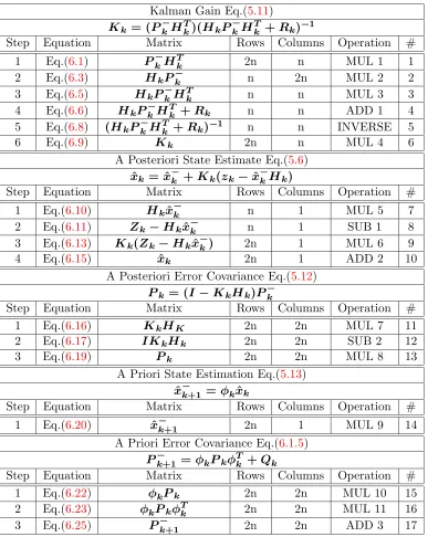
5.4 Kalman filter matrix operations . . . 91

6.1 Maximum PMC readings for both algorithm versions . . . 109

6.2 Selected PIII PMC Events for Experiment . . . 118

6.3 Examples of MESI related PMC events . . . 122

7.1 Testbed Machines for the Kalman Filter Evaluation . . . 123

8.1 Measurement Vector Structure for the C2STATE Algorithm . . . 137

A.1 PIII Performance Monitoring Counters Description . . . 156

(17)

βi Time constant for a particular PMC process, see equation (5.20), page 70

∆t Sample interval, see equation (2.1), page 35

∆tmin Minimum sample interval, see equation (2.1), page 35

1

β Time constant in exponential autocorrelation function for Gauss-Markov process, see equation (5.15), page 69

ˆ

RX(τ) Estimated autocorrelation function, see equation (5.25), page 71 ˆ

RX(n∆t) Discrete estimated autocorrelation function, see equation (5.25), page 71

σ2 Variance in exponential autocorrelation function for Gauss-Markov process, see equa-tion (5.15), page 69

σ_i2 Variance for a particular PMC process, see equation (5.20), page 70

τ Autocorrelation time difference variable, see equation (5.25), page 71

e(t) Mean of the counted events e(t) over the sample interval ∆t, see equation (2.1), page 35

RX(τ) Autocorrelation, see equation (5.15), page 69

T Autocorrelation time interval, see equation (5.25), page 71

tk Sample time, see equation (5.2), page 65

u(t) Unity white noise in continuous state space model, see equation (5.16), page 69

X(t) Stationary Gaussian process, see equation (5.14), page 69

x1 Integrated Gauss-Markov process in continuous state space model, see equation (5.16), page 69

x2 Gauss-Markov process in continuous state space model, see equation (5.16), page 69

(18)

ˆ

x−

k A Priori state vector, see equation (5.14), page 68

ˆ

xk Estimated state vector, see equation (5.2), page 65

φk State transitions matrix, see equation (5.2), page 65

e−

k = Estimation error, see equation (5.5), page 67

H Measurement sensitivity matrix, see equation (5.2), page 65

Kk Kalman Gain, see equation (5.2), page 65

Pk A Posteriori error covariance matrix, see equation (5.8), page 67

P−

k A Priori error covariance matrix of the estimated state vectorxˆ−k, see equation (5.8), page 67

Qk Process noise covariants matrix, see equation (5.2), page 65

Rk Measurement noise covariance matrix, see equation (5.5), page 67

vk Measurement noise is described by the covariance matrix Rk, see equation (5.3), page 66

wk Sequence with a covariance determined by the covariants matrix Qk of the process noise associated with the system’s state dynamics, see equation (5.2), page 65

(19)

AGP Accelerated Graphics Port

AKF Adaptive Kalman Filter

AMBA Advanced Microcontroller Bus Architecture

API Application Programming Interface

ASIC Application Specific Integrated Circuits

ATM Asynchronous Transfer Mode

Blink Backside Link

C2STATE Compute Cluster State Estimation

CCA Common Component Architecture

ccNUMA cache-coherent None-Uniform Memory Access

CPU Central Processing Unit

DCU Data Cache Unit

DDR Double Data Rate

DIRA Divided-Interval Rectangular Area

DMA Direct Memory Access

DSM Distributed Shared Memory

DSP Digital Signal Processing

DVI Digital Visual Interface

DVS Dynamic Voltage Scaling

(20)

EISA Extended Industry Standard Architecture

EKF Extended Kalman Filter

ESA European Space Agency

FDDI Fiber Distributed Data Interface

FIFO First In First Out

FPGA Field Programmeable Gate Array

FSB Front-Side Bus

GALS Globally Asynchronous Locally Synchronous

gcc GNU Compiler Collection

GIDS Grid-wide Intrusion Detection System

GNU GNU’s Not Unix

GPS Global Positioning System

GPU Graphics Processing Unit

GUI Graphical User Interface

HDL Hardware Description Languages

I/O Input/Output

IC Integrated Circuits

IEEE Institute of Electrical and Electronics Engineers

IFU Instruction Fetch Unit

IKF Interval Kalman Filter

ILP Instruction Level Parallelism

IPC Instructions Per Cycle

IQ Issue Queue

KVM Keyboard Video Mouse

L1 Level 1 Cache

(21)

LC2 Link Controller 2

LC3 Link Controller 3

LC Link Controller

LSQ Load/Store Queue

LVDS Low Voltage Differential Signalling

MCD Multiple Clock Domain

MDL Metric Description Language

MESI Modified Exclusive Shared Invalid

MIT Massachusetts Institute of Technology

MLR Multiple Linear Regression

MMSE Minimum Mean-Square Error

MPI Message Passing Interface

MPP Massively Parallel Processing

NFS Network File System

NUMA Non-Uniform Memory Access

ODBC Open DataBase Connectivity

OS Operating System

PAL Programmable Array Logic

PCB Printed Circuit Board

PCI Peripheral Component Interconnect

PCL Performance Counter Library

PC Personal Computer

PDF Probability Density Function

PDT Program Database Toolkit

PIO Programmed Input Output

(22)

PLB Pipeline Balancing

PMC Performance Monitoring Counter

PME Positional Mean Error

PVM Parallel Virtual Machine

ROB Reorder Buffer

SANTA System Area Network Trace Analysis

SCAAT Single-Constraint-At-A-Time

SCI Scalable Coherent Interface

SFI Science Foundation Ireland

SISCI Software Infrastructure for Scalable Coherent Interface

SMP Symmetric Multiprocessor

SQL Structured Query Language

SRAM Static Random Access Memory

TAM Trapezoid-area Method

TCD Trinity College Dublin

TSC Time-Stamp Counter

VHDL (VHSIC) Hardware Description Language

VHSIC Very High Speed Integrated Circuit

(23)

Introduction

This thesis is concerned with the architectural organisation, the performance measurement and the real-time performance estimation of hardware DSM clusters. These machines may incorporate various subsystems, e.g. Central Processing Unit (CPU)s, GPUs, Chip-sets, FPGAs and interconnect interfaces. It is the objective of the performance estimation to provide a global view of the computational state of all these subsystems throughout the cluster. In order to facilitate real-time performance estimation research and investigations into novel high performance hybrid graphics cluster architectures, a general-purpose testbed cluster was built from commodity components and a second special-purpose hybrid system was designed. Both systems employ the Institute of Electrical and Electronics Engineers (IEEE) 1596-1992 Scalable Coherent Interface (SCI) [Ins93] as interconnect. This technology provides DSM in hardware and allows for the configuration of Non-Uniform Memory Access (NUMA) and cache-coherent None-Uniform Memory Access (ccNUMA) clusters.

1.1

Non-Invasive Trace Data Acquisition of SCI Hardware

DSM Interconnect Traffic

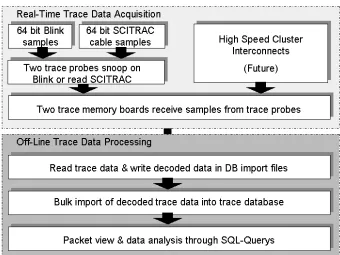
Initial investigations with Dr. Brian Coghlan into the non-intrusive acquisition of SCI inter-connect traffic [MC99a] provided an understanding of their true communication statistics. This work required the design and construction of hardware and software for the non-invasive acquisition of interconnect traffic at real-time and the subsequent off-line trace data analysis. This infrastructure is shown in Fig.2.2.

(24)

1.2

Global Real-time Estimation of Incomplete Performance

Measurements

Subsequent work focused on a novel approach to estimating and predicting the DSM system-wide utilisation of computational resources in real-time [MC05a]. An algorithm that imple-ments a Discrete Minimum Mean-Square Error (MMSE) Filter is applied to fuse concurrent and sequential observations of system event counts into the filter’s state vector. Contem-porary computer components and subsystems make these event counts available through hardware PMC registers. The registers may be accessed by the system’s software quasi-concurrently1 but the number of registers in individual components is usually smaller than the number of events that can be monitored. This approach overcomes this problem by modelling individual hardware PMC readings as vector random processes and recursively processes them one (or a group) at a time into a common state vector, thereby making larger performance counter sets observable than would otherwise be possible.

This algorithm can be applied to fuse various PMCs from a single node or a set of compute cluster nodes. The memory hierarchy of a hardware DSM cluster is in this context of particular interest because load and store operations trigger PMC events that indicate cache and memory activity. Furthermore, a memory reference made to a remote memory causes counter events on the DSM’s interconnect interface cards. The algorithm allows us to merge all this information into a common state vector. Consequently this approach allows us to observe the entire system state at real-time from any node in the system.

1.3

Special Purpose High Performance Graphics DSM

Clus-ter

Work on the non-invasive measurement and analysis of high speed interconnect traffic and investigations into the global state estimation of compute clusters led to the conceptual de-sign of a special-purpose high-performance graphics cluster [MBO+06]. Section 7.2 of this thesis describes the design of this scalable tightly coupled cluster of custom-built boards that provide an Accelerated Graphics Port (AGP) interface for commodity graphics accel-erators. These boards are supplied with rendering instructions by a cluster of commodity Personal Computer (PC)s that execute OpenGL graphics applications. All the commodity PCs and custom-built boards are interconnected with an implementation of the SCI stan-dard. This technology provides the system with a high bandwidth, low latency, point to point interconnect. The design allows for the implementation of a 2D torus topology with good scalability properties and excellent suitability for parallel rendering. Most importantly the interconnect implements a DSM architecture in hardware. Figure 7.7 shows how local

1_{The reading of several PMC registers is considered as a concurrent operation because the amount of time}

(25)

memories on the custom-built boards and the PCs become part of the system wide DSM. Figure7.7also depicts FPGAs on the custom-built boards. These reconfigurable components assist the SCI implementation and provide substantial additional computational resources that may be used to control the commodity graphics accelerators and to perform operations associated with a parallel rendering infrastructure, or even ray tracing and physics simula-tions. These reconfigurable components are an integral part of the scalable shared-memory graphics cluster and consequently, increase the programmability of the parallel rendering system just like vertex and pixel shaders increased programmability of graphics pipelines. The implementation and investigation into the opportunities provided by this design will be investigated as future work. The global performance estimation algorithm will be integrated into the graphics cluster to investigate its suitability for load balancing.

1.4

Contributions

The main contribution is this work is the global real-time performance state estimation of DSM clusters. To the best of my knowledge nobody has investigated the suitability of MMSE Filters to observe a large number of PMC readings that would otherwise be unobservable. Further contributions are the non-invasive acquisition and analysis of SCI interconnect traffic and the application of interconnect traffic statistics to tune network simulations. All this work was published in international peer reviewed conferences [MC05a, MKCL01,MC99a] and a list is provided in section1.4.2.

My conceptual design of the graphics cluster is the predominant part of a successful Science Foundation Ireland (SFI) Basic Research Grant proposal [OMK04] written in col-laboration with the Principal Investigator (PI) Dr. Carol O’Sullivan and Dr. Anil Kokaram, both of Trinity College Dublin (TCD). The following three quotations are from the rigorous peer review:

A well written and well thought through proposal. The research is very far-sighted, and considerable ingenuity has been applied to obtain a cost-effective solution to the graphics speed problem.

If successful, the project outcomes would make an important contribution to the field.

Overall though this is a very strong, well thought out proposal, based on a very good and novel idea.

(26)

1.4.1 Thesis Statement

Data fusion of sequential and concurrent Performance Monitoring Counter (PMC) readings with Minimum Mean-square Error (MMSE) algorithms allows for the estimation of the computational state of Distributed Shared Memory (DSM) clusters. These PMC readings could otherwise not be observed with a comparable accuracy.

1.4.2 Directly Relevant Peer Reviewed Publications

[MBO+₀₆_] _{Michael Manzke, Ross Brennan, Keith O’Conor, John Dingliana, and Carol}

O’Sullivan. A scalable and reconfigurable shared-memory graphics architecture. In

Proceedings of the SIGGRAPH 2006 Conference on Sketches & Applications, 2006

[MC05a] Michael Manzke and Brian A. Coghlan. Optimal performance state estimation

of compute systems. In the Proceedings of the 13th IEEE International Symposium on Modeling, Analysis, and Simulation of Computer and Telecommunication Systems (MASCOTS 2005), pages 511–516, September 2005

[MKCL01] Michael Manzke, Stuart Kenny, Brian Coghlan, and Olav Lysne. Tuning and

verification of simulation models for high speed interconnection. InPDPTA’2001, June 2001

[MC99a] Michael Manzke and Brian Coghlan. Non-intrusive deep tracing of sci interconnect

traffic. In Wolfgang Karl and Geir Horn, editors,SCI Europe ’99, pages 53–58. SINTEF Electronics and Cybernetics, September 1999. ISBN 82-14-00014-9

1.4.3 Indirectly Relevant Peer Reviewed Publications

[MB04] Michael Manzke and Ross Brennan. Extending fpga based teaching boards into the area of distributed memory multiprocessors. InWorkshop on Computer Architecture Education, pages 15–21, June 2004

(27)

1.5

Thesis Organisation

This thesis is organised as follows:

Chapter 1 Introduction provides a general introduction to the main research questions

that were investigated as part of this thesis. This includes a description of the contribution in section 1.4, the thesis statement and lists of directly and indirectly relevant publications in section 1.4.2and section1.4.3respectively.

Chapter 2 Motivation discusses the motivation for the main investigations that were

conducted. In section 2.2 an argument to model PMC readings as random processes and to apply a discrete MMSE filter to fuse these PMC readings into common state vector is presented. At the beginning of this chapter in section 2.1 and section 2.1.1 a non-intrusive SCI trace instrument and its associated analysis software is introduced. Section 2.1.2then elaborates on how trace data from the SCI Deep Trace instrument may be used to tune and validate SCI network models. It is pointed out that the non-intrusive acquisition of SCI network traffic and the tuning of SCI network models based on these trace data led to the idea to model PMC readings as random processes. Section 2.3 makes an argument for the advantages of Kalman filters to fuse many sequential PMC readings. This notion is expanded in section2.4to a distributed implementation that allows for the global observation throughout the nodes in hardware DSM clusters. The last section 2.5 in the motivation chapter2looks at the design of a special purpose graphics cluster. This design was strongly influenced by the previously mentioned investigations.

Chapter 3 Background and Related Work provides an introduction to the SCI

tech-nology in section 3.4.2. This is followed by related work descriptions for the main research questions. Section3.2presents related work for the “Trace Data Acquisition”, section 3.3.1

for the “MMSE Filter”, section 3.1.1 for “Performance Monitoring Counters”, section 3.1

for “Performance Analysis” and section3.5 for the “Special Purpose Graphics Cluster”.

Chapter4 High Speed Interconnect Trace Data Aquisition and Analysis provide

a detailed discussion of the non-invasive high speed interconnect trace data acquisition and analysis. Section 4.4 describes how a SCI network model may be tuned and validated with interconnect statistics acquired with the trace instrument from section 4.1, section 4.2 and section4.3.

Chapter 5 State Estimation of a Single Compute Node is dedicated to the main

(28)

estimation algorithm. The last two sections of the chapter deal with the fusing of PMC reading sets into a larger state vector and with the implementation of the algorithm. This is discussed in section5.3 and section5.4respectively.

Chapter 6 Optimisation and Re-evaluation of the Estimation Algorithm

dis-cusses some of the possible optimisations for the estimation algorithm in section 6.1 and analyses these in section 6.2. This is followed by an extended evaluation of the estimation algorithm for a single-node system in section6.3 and section6.4.

Chapter7 Hardware DSM Testbeds provides a detailed description of two multi-node

testbeds. One is a loosely coupled DSM cluster that is the testbed for all the implementations and evaluations in this thesis. This cluster is discussed in section7.1. The second cluster is a conceptual design of a tightly coupled special purpose high performance graphics cluster. This cluster will eventually take full advantage of the estimation algorithm by using it for load-balancing. This tightly coupled cluster is described in section 7.2

Chapter 8 Compute Cluster State Estimation Algorithm (C2_STATE) _finally

ap-plies the estimation algorithm to hardware DSM systems. Section8.1describes the necessary alterations to the single-node estimation algorithm and section8.2presents experiments and evaluation results of the global state estimation algorithm (C2_STATE).

Chapter 9 Conclusions and Future Work section 9.1summarises the work presented

(29)

Motivation

Clusters of commodity PCs have become a dominant alternative to Massively Parallel Pro-cessing (MPP) systems. TheTop 500 Supercomputer list included 28 clusters and 346 MPP systems in November 2000. In November 2005 this had changed to 360 clusters and 104 MPP systems [Sit05]. The majority of these clusters are loosely coupled systems that ex-hibit reasonably high bandwidth but relatively long latencies. They are not really suitable for fast real-time applications.

Interconnect technologies enable us to connect uniprocessors or Symmetric Multipro-cessor (SMP) machines into clusters. This technology determines how tightly or loosely coupled a cluster is. This thesis focuses on a particular subset of clusters that implement DSM in hardware. Within this scope, the work investigates hardware DSM systems that are completely assembled from commodity components as well as systems that employ some built components, thereby filling the void in the design space between fully custom-built high performance systems and systems that are entirely constructed from off-the-self components.

(30)

In this thesis I have chosen the SCI interconnect technology because it allows for the design of hardware DSM clusters that explicitly reduce latencies. In order the take full advantage of various computational resources provided by a hardware DSM cluster and to reduce the power dissipation of these clusters, one can employ various optimisation tech-niques. All these optimisations require run-time performance measurements.

This thesis describes two novel performance measurement and analysis methodologies that can be used to exploit any of these optimisations. The first method is concerned with the non-intrusive acquisition of interconnect traffic, which can assist the design and the verification of SCI based hardware DSM clusters. It allows the analysis of whether the interconnect topology can meet bandwidth and real-time constraints. It also helps to pinpoint bottlenecks in the interconnect topologies. The second method, the global state estimation of hardware DSMs, can control runtime adaption whether in hardware or software. The bulk of this thesis concentrates on this second method.

This thesis also discusses the conceptual design of a special-purpose tightly coupled hard-ware DSM system that can drive large scale interactive visualisation systems. This design is intended as a future target for the non-intrusive acquisition of SCI interconnect traffic and execution of the global state estimation algorithm.

2.1

Trace Data Acquisition and Analysis

The observation of high speed interconnect traffic, such as SCI, requires either to take mea-surements on the interconnect cable or to perform these meamea-surements on the interface-adapter. Both methods have advantages and disadvantages that will be discussed later. In section 4.1 and section 4.2 an instrument and the associated software infrastructure is described that acquires interconnect traces and deposits these time-stamped and decoded traces into a database for subsequent analysis. Section4.4discusses how the instrument and software infrastructure may be used to tune a SCI fabric simulation model.

2.1.1 The SCI Non-Intrusive Deep Trace Instrument and Analysis

Infras-tructure

(31)

[image:31.595.147.487.109.364.2]

Figure 2.1: Trace data flow overview

The primary observation of interface traffic is accomplished through snooping on the Back-side Link (Blink) [Dol96], Dolphin’s implementation of the SCI transfer cloud. Snooping on SCI cable traffic, via SCILAB’s SCITRAC [SBNW98], is also supported. The tracer’s configuration consists of three modules, a trace probe, a deep trace memory and a trace database. The database provides a powerful means for a fine-grained analysis of a large quantity of trace data.

The instrument provides hardware designers and software developers with a tool that allows a deeper understanding of the temporal behaviour on any given target system. Unlike other systems, e.g. see [KL97, KLS99], this trace instrument is targeted to commercially available interconnect hardware and therefore provides the user with information about the true temporal behaviour of clusters made up of standard components. Fig. 2.1 shows how the trace instrument’s hardware and software components are related to each other during trace data acquisition and subsequent off-line data analysis.

The instrument is designed to fulfil the following main objectives:

• Non-intrusive monitoring of SCI interconnect traffic

• Very deep ( 10Mbyte) interconnect traces per node

• Acquisition of all the interconnect traffic

(32)

• Allowance for various probes to accommodate SCI cable traffic and Blink traffic

• Straightforward adaptation to various SCI interface implementations.

• Trace data storage in commercial relational database

• Ability to analyse causal relationships in synchronously acquired traces from different targets

The utilisation of a relational database provides the user with an easy means to extend and to adapt the predefined database queries to their specific needs.

2.1.2 Tuning and Validation of SCI Network Models through Non-Intrusive

Deep Traces

The non-intrusive acquisition of interconnect trace data and a subsequent data analysis can be used to accurately tune the definition of interconnect loads and the parameterisation of interconnect simulation models. High speed interconnects or system area networks are the principal components of a compute cluster that transform stand alone computers into a clus-ter. The design of such interconnect fabrics may be assisted through performance prediction. This prediction is accomplished through simulation if the model’s parameterisation reflects the physical fabric and realistic load descriptions are provided.

A simulation is only as accurate as its simulation model. A simulation model must be tuned and verified in order to guarantee that the model reflects the real physical system behaviour, but this requires information about the true temporal behaviour of the physical interconnect. This information can be extracted from interconnect trace data. In particular, the trace data must be acquired non-invasively for it to be accurate.

(33)

Figure 2.2: Trace Data Acquisition and analysis framework

2.2

Global State Estimation of Hardware Distributed Shared

Memory (DSM) Systems

Today’s high performance computers, whether uniprocessor, multiprocessor or hardware DSM systems, are madeup of concurrently operating subsystems. Run-time knowledge of the system-wide utilisation state of these subsystems including CPUs and their interconnects can assist efficient scheduling of tasks onto these resources. E. Duesterwald et al. [DCS03] argue for a prediction that would allow the system to adapt more efficiently to the time-varying behaviour of the programs. Their work observes performance metrics that are based on CPU PMC event readings. An analysis of these observations showed that programs exhibit strong behaviour variations at PMC sample interval granularity but that the various metrics shared periodicity. E. Duesterwald et al. [DCS03] exploit this characteristic to perform resource-aware scheduling.

(34)

gen-eral purpose processor through Pipeline Balancing (PLB). In this case performance mon-itoring controls the dynamic adaption of resources. Dynamic program phase detection is applied in Balasubramonian et al. [BABD00] to optimise the memory hierarchy configura-tion. This leads to a lower power dissipation and improved performance. Balasubramonian et al. [BDA03] investigate optimisations of clustered micro-architectures [FCJV97,PJS97]. This is accomplished by taking advantage of Instruction Level Parallelism (ILP). For clus-tered micro-architectures the optimal performance is achieved by finding the best trade-off between communication and parallelism. Again program phases are detected to adapt the cluster configuration to the current workload. In Dhodapkar and Smith [DS02] a recon-figurable instruction set cache is adapted by matching working set signatures with current program phases. Folegnani and Gonzales [FG01] lower the energy consumption of the CPU’s issue logic by dynamically reducing the effective size of the instruction queues. Huang et al. [HRT03] propose an alternative to the temporal approach to adaption. They use subrou-tines at the granularity of program phases to determine the correct adaption of the system. Dynamic Voltage Scaling (DVS) is used by Hughes et al. [HSA01] to adapt general-purpose processors to multimedia workloads that operate on per frame time constraints. Magklis et al. [MSS+03] investigate DVS techniques in Multiple Clock Domain (MCD) micro-architectures. These target systems operate with Globally Asynchronous Locally Synchronous (GALS) clocks that are dynamically scaled relative to queue utilisation. These queues supply clock domains with data or instructions. Similar to Folegnani and Gonzales [FG01], Ponomarev et al. [PKG01] adapt the length of the Issue Queue (IQ), the Reorder Buffer (ROB) and the Load/Store Queue (LSQ) depending on their occupancies. Finally, Wu et al. [WMC+05] explore a dynamic compilation environment to control DVS.

In addition to the dynamic adaption work, researchers have successfully investigated PMC events to predict the run-time CPU and memory power consumption [IM03, Bel00,

Mar01,KCK+01,LJ03]. Contreras and Martonosi [CM05b] used a first-order, linear power estimation model to observe CPU and memory power consumption based on PMC readings. All these research activities are good examples of the wealth of optimisation opportunities that are available if dynamic adaption or scheduling is employed. It also illustrates that the ability to indirectly measure power consumption in parts of the CPUs micro-architecture is useful if energy is to be saved. Furthermore all the work cited here depends on accurate PMC event readings. This emphasises the importance of accurate counter readings of a variety of events.

This thesis is not concerned with the scheduling of resources, the dynamic optimisations or the measurement of power consumption, but introduces an algorithm that generates a global view of the system’s utilisation or computational state. It is for other to use these state information for optimisations. The global view is derived from hardware PMC readings that count the number of occurrences of a selected event.

(35)

e(t) over the sample interval ∆t. The choice of duration of the sample interval ∆t is a trade-off between counter accuracy and computational overhead. Reducing ∆twill increase the accuracy until the computational overhead (caused by instructions that read and pro-cess the PMC registers) contributes a significant amount of counter events to the reading. Section5.4provides a detailed discussion of this topic. Furthermore if the system’s software is responsible for the acquisition of counter readings then the Operating System (OS) ability to schedule such register readings determines the minimum sample interval ∆tmin.

zk= 1 ∆t

(k∆t)+∆t

X

k∆t

e(t) (2.1)

System events, such as the Number of Instruction Fetch Misses, that are counted over a time period provide a measurement of the degree of availability or utilisation of particular system resources. These observations are easily obtained through registers that implement performance counters. In general counter registers can be instructed to count a particular event by means of a selection register. This selection is required because in most cases the number of PMC registers does not match the number of events that may be counted. For example theIntelTM_PIII _{processor has only two registers but each of these may be used to}

count any one of more than 100 events ranging from theNumber of Bus Transactions to the

Number of Floating-point Operations [Ord01]. Please see TableA.1 for a complete list of all available PMCs.

This selection approach does not constitute a problem as long as the number of required PMC readings does not exceed the number of available counter registers. If the number of distinct event counts exceeds the number of available registers then this approach fails. One remedy is if the system uses a single register to count different events in a nested sequence. Fig.2.3depicts this multiplexing technique. Aset in Fig.2.3refers to the number of PMC registers in a given subsystem. The shaded areas in this figure highlight the intervals [∆t2,∆tn] and [∆tn+2,∆tn+n], withn as the total number of event sets required to observe the current state of resource utilisation. No events are counted for the first counter set, and consequently the accuracy decreases for these multiplexed readings [DLM+₀₁_].

(36)

∆tn+n ∆tn+2

∆tn+1 ∆tn ∆t2

∆t1

First Set of Counter Samples Second Set of Counter Samples

Last Set of Counter Sample

Figure 2.3: Multiplexed sets of performance counter readings

2.3

MMSE Filter Algorithm

The discrete MMSE filter was originally formulated by R. Kalman in 1960 [Kal60] and can process multiple time-variable inputs through the use of state space methods. The application of stochastic system models for the PMC event readings is not only beneficial for the optimal estimation of a noise-corrupted and incomplete scalar reading but also for multiple readings. This thesis demonstrates how the well known Kalman filter algorithm can be used to make a larger variety of PMC information accessible to the system’s software than would otherwise be observable with a restricted number of counter registers.

Fundamental to the Kalman filter is the presence of noise. In this particular case, the noise originates from the non-deterministic execution of the PMC acquisition software. The histogram in Fig. 2.4 shows how the sample time changes around the mean of 3.9532e+07 clock cycles. The CPU operates at 1 GHz, consequently the mean sample time of 3.9532e+07 clock cycles is equivalent to 39.532 ms. The samples vary with a standard deviation of

σ = 1.1074e+ 5 around the mean. Section 5.1.2 shows that the state transition matrix Φ and the covariance matrix Q of the Kalman filter algorithm both depend on the sample interval ∆tbut the filter operates with a fixed sample time. Therefore the filter will process randomly too many or too few PMC events. This is seen from the filter’s perspective as noise. A further contributing factor is the quantisation of the PMC event readings.

2.4

Distributed MMSE Filter Algorithm

(37)

0 1e-06 2e-06 3e-06 4e-06 5e-06 6e-06

3.88e+07 3.9e+07 3.92e+07 3.94e+07 3.96e+07 3.98e+07 4e+07 4.02e+07

Number of samples

Sample Time [clock cycles]

Sample Time Histogram with superimposed Gausian PDF sigma = 1.1074e+05

mean = 3.952e+07 clock cycles = 0.039532 sec

Histogram Gaussian PDF

Figure 2.4: Sample Time measured on CPU 1 in one of the two SMP systems specified in table 7.1

are suitable for a run-time performance analysis. I have named this algorithm the “Compute Cluster STATE estimation” (C2_{STATE) algorithm. Every node in the cluster that requires} a global performance view runs a MMSE filter algorithm that fuses local and remote PMC readings into its state-vector. From the perspective of each node, remote PMC readings are made available through the shared memory. Consequently all participating nodes hold an estimate of the cluster wide performance in state space representation. This state-vector may be used for performance measurements, load balancing and other optimisations.

2.5

Special-Purpose Graphics Cluster

(38)

motion tracking and other I/Os to provide feedback to the application. To guarantee a seamless integration of this information into the interactive application it is necessary to limit the latencies involved. One advantage of the SCI interconnect is that it operates at extreme low latencies especially if an I/O bus is avoided.

(39)

Background and Related Work

This thesis is concerned with the global state estimation of hardware DSM clusters. The work also presents a novel special purpose hardware DSM architecture that is intended to employ the global state estimation algorithm to optimise its performance. This chapter provides the background to this work and discusses related work.

3.1

The Performance Analysis

In general performance analysis comprises the measurement of performance data, the eval-uation of these data and a subsequent optimisation. The evaleval-uation and optimisation may be performed off-line or at run-time. Performance analysis can also be divided into: per-formance measurement, perper-formance modelling and perper-formance simulation. This thesis focuses on the measurement and estimation of DSM performance but also discusses possible applications.

There are several commercial and research tools for the performance analysis of paral-lel applications. They are suitable for message passing and shared memory programming paradigms. The performance measurements are derived from system event counts. These may be based on hardware or software event counts. Hardware events are implemented within PMC registers. Software events require the instrumentation of the source or ob-ject code. These event counts are then used for profiling or tracing. In the case of profiling, statistics for several event-counts are generated. Tracing requires the acquisition of the event history. This approach generates large quantities of trace data that are usually analysed after the execution of a parallel program.

Some manufacturer of parallel high performance systems provide performance analysis tools for their systems. IBM’s XProfiler allows for the profiling of serial and parallel applica-tions [Xpo06]. Similar features are included in SGI’s ProDev WorkShop [Pro06] and Cray’s PAT [GM98,PAT06].

(40)

Ana-lyzer Collector [Tra06]. Other third party tools such as ETNUS’ Totalview include Message Passing Interface (MPI) [Mes03] and OpenMP [Ope05] debugging tools [Tot06]. As with To-talview, Crescent Bay Software’s Deep [Dee06] supports the debugging of message passing and shared memory machines, but this tool also uses PAPI [PAP02] to gain access to PMC readings. The “European Center for Parallelism of Barcellona” has developed the Paraver tools with similar functionality [JJLG03,GTAB01,JJL+03,FCL02].

The TAU project [Tau06] provides profiling and tracing for performance analysis of par-allel programs. Performance measurements are achieved through the instrumentation of source code and use of a Program Database Toolkit (PDT), see Lindlan et al. [LCM+00]. The framework can also dynamically instrument the binaries by using Paradyn’s DyninstAPI (see later). The PDT database holds compile-time information for source-level feedback. Malony et al. [MST+₀₅_{] discuss the integrated measurement, monitoring, and optimisation}

of Common Component Architecture (CCA) component-based applications.

(41)

pro-pelled dynamic instrumentation agent that searches for intermittent performance problems. Harris and Miller [HM05] present content and structure analysis methods that can deal with stripped binary code. Collins and Miller [CM05a] discuss a search techniques for fine-grained program structures in order to efficiently instrument loops. Roth and Miller [RM06] present a bottleneck detection strategy for systems that run a large number of processes. They achieve this by applying a novel multicast and data aggregation infrastructure.

The TAU and Paradyn projects are a good examples of very productive long-term re-search activities.

3.1.1 Performance Counter

Most contemporary CPUs have hardware PMC registers that may be sampled to derive performance information about the CPU’s micro-architecture. Access to these registers may be provided through high level APIs, e.g. Performance Counter Library (PCL) [PCL06] and PAPI [PAP02]. These high level APIs are also used by many of the previously mentioned performance analysis tools, e.g. TAU. A number of publications relate to the widely used PAPI API [MDK+04,AM05,DMM+04,DBL,DMM+03,DLM+03,WM03]. These two APIs use Mikael Pettersson’s Linux 2.x.x kernel patch [Pet02] to access Intel Pentium, Pentium MMX, PPro, Pentium II, Pentium III, Pentium 4 and AMD Athlon, Duron PMCs in kernel space.

Ojha [Ojh01] compares hardware PMC measurement with software and hybrid perfor-mance counters. Moore [Moo02] compares the PMC counting and sampling modes. C´erin and Fkaier [CFJ03] investigate sorting algorithms by observing the ratio of L1 data cache misses and retired instructions through PMC readings. This work uses Mikael Pettersson’s “perfctr” [Pet02].

3.1.2 Multiplexed Performance Counter Readings

Many performance measurement situations require the reading of more PMC events than can be simultaneously sampled with the number of available PMC registers. One solution is to multiplex PMC events onto the PMC registers at the expense of accuracy. For example PAPI uses the MPX [May01] library to implement multiplexing. Mathur and Cook [MC05b] in-crease the accuracy of multiplexed PMC readings by applying Positional Mean Error (PME), Multiple Linear Regression (MLR), Trapezoid-area Method (TAM) and Divided-Interval Rectangular Area (DIRA) estimation methods. Azimi et al.[ASW05] improves multiplexing accuracy through high frequency PMC sampling. This is possible with the K42 research OS [SKW+06].

3.1.3 Cluster wide PMC Collection

(42)

3.2

Trace Data Acquisition and Analysis Related Work

Hollingsworth et al. [HLM95] discuss various techniques for performance measurement of parallel systems. The authors distinguish between program instrumentation and hardware instrumentation. They point out that the instrumentation of executables may perturb the execution of a parallel program but that hardware instrumentation is non-intrusive. Despite this obvious advantage the hardware instrumentation makes it difficult to associate hardware based performance information with the source code of the executed program. The authors suggest that a hybrid solution can provide a trade-off between the non-intrusion nature of the hardware instrumentation and the software instrumentation ability to provide performance data that are easily associated with the source code. They also argue that a hardware instrumentation must be distributed over all the nodes in the system.

Martonosi et al. [MCM96] presents Princeton’s SHRIMP performance monitor and pro-vides a detailed discussion of the hardware monitor. An FPGA-based monitor is attached to each node in the SHRIMP system and accumulates interconnect events. The monitor cards also support multiplexing.

An alternative solution is provided by Liao et al. [LJI+₉₈_{]. The authors utilise the}

programmable network interface card of a Myrinet-based cluster to implement a performance measurement mechanism. This approach uses a software solution but implements it on an independent platform.

Karl et al. [KST00] reports about a hardware monitor similar to Princeton’s SHRIMP performance monitor. The monitor hardware is attached to SCI interface cards on every node in the cluster and snoops on the local bus of the interface card. Interconnect events are stored through a caching mechanism that increases the utilisation of the available event memory [HJK+00,TGS+01,GST+02,KLS99].

More recently Kenny et al. [KCB+₀₅_{] investigated Ethernet traffic performance analysis.}

The authors used features of the interface card to collect and analyse Ethernet traffic that is specific to grid operations.

3.3

Kalman Filtering

(43)

filtering.

The filter has been applied in many areas: Chen et al. [CWS97] propose an Interval Kalman Filter (IKF) for the estimation of interval linear systems. Pearson et al. [PGEM97] investigate the stability of combat aircraft Extended Kalman Filter (EKF)s for high system integration. Hong et al. [HCC98] use discrete wavelet transforms that are implemented on a Kalman filter bank to decompose multiresolutional random signals. McMillan et al. [McM94] compares Kalman filter estimates that are based on Global Positioning System (GPS) re-ceivers with estimates that are based on inertial equipment. The measurements were con-ducted during sea tails. Kuo et al. [KHJ+96] propose a block-based motion estimation method that uses a Kalman filter to assist the compression of video signals. Murty and Smolinski [MS88] apply a five-state Kalman filter to estimate the fundamental and second harmonic of a power system in order to implement a digital differential relay for a three phase power transformer. Sinopoli et al. [SLF+04] use a Kalman filter to model the arrival of observations as a random process. These observation originate from unreliable commu-nication channels in large, wireless, multi-hop sensor networks. These example demonstrate the diversity of applications of the Kalman filter.

3.3.1 MMSE Filter Related Work

In the Computer Science domain there are also many examples of Kalman filtering. Discrete MMSE filters were investigated for network traffic flow control [Kes91] and motion tracking applications [Bac00][Gre96] but, to my knowledge, they were not investigated for the acquisi-tion of PMC readings. Gregory Welsh developed the Single-Constraint-At-A-Time (SCAAT) solution for motion tracking with an EKF[Gre96].

3.4

Compute Cluster

According to the Top 500 Supercomputer list [Sit05] clusters have became the most used systems for high performance computations. The list included 28 clusters and 346 MPP systems in November 2000. In November 2005 this had changed to 360 clusters and 104 MPP systems [Sit05].

3.4.1 Interconnect Technologies

(44)

3.4.2 Scalable Coherent Interface (SCI)

Defined in 1992, SCI is a well established technology and many high performance cluster im-plementations employ this interconnect (e.g, PC2 University of Paderborn Germany, Univer-sity Of Delaware - The Bartol Research Institute USA and National Supercomputer Centre in Sweden) [Top04]. Subsets of the SCI standards have been implemented and are avail-able as commodity components. In particular, Dolphin [Dol04] has implemented Peripheral Component Interconnect (PCI) cards that bridge PCI bus transactions to SCI transactions. Hellwagner et al. [HR99] cover much of the related hardware and software. Compute nodes with PCI slots may be interconnected through PCI-SCI bridges together with a suitable SCI fabric topology, thus bridging their PCI buses. Memory references made by one of these nodes into its own PCI address space are translated into an SCI transaction and transported to the correct remote node. The remote node translates this transaction into a memory access, thus providing a hardware DSM implementation. Programmed Input Output (PIO) and Direct Memory Access (DMA) may be performed without the need for system calls.

Figure 3.1 illustrates the design of a Symmetric Multiprocessor SMP node with a com-modity SCI card in one of its PCI slots and also shows the main components on this SCI card. The PCI-SCI bridge translates between PCI transactions and SCI transactions and forwards them onto the PCI bus or the Blink bus. The SCI Blink bus interconnects the PCI-SCI bridge with up to seven SCI Link Controller (LC)s or alternative components. The SCI cards shown have two SCI LCs attached to the Blink and consequently are suitable for the construction of a 2-dimensional torus. Systems with more than one LC route packets between them over the Blink to the corrected LC according to a routing table. This enables distributed routing of SCI packets between individual SCI rings without an expensive central SCI switch. Routing is configured during SCI fabric initialisation. Every LC has an input and output port, and the output port of one is connected via a cable to the input port of another. These links are 16 bit parallel and unidirectional with a bandwidth of 667Mbytes/s.

SCI and Cache Coherency

(45)

Intel

SCI Link Controller ONE

SCI Link Controller TWO PCI

PCI

SCI Card Commodity

North Bridge Memory

Commodity SMP PC Application Operating System CPU 2

Graphics Application

Operating System CPU 1

Graphics

Bridge

SCI BLink

Figure 3.1: SMP Desktop Node with 2D SCI-PCI interface card.

SCI Commodity System Software

SCI driver software and a Software Infrastructure for Scalable Coherent Interface (SISCI) API for the Dolphin SCI cards force the OS to reserve a particular section of the main memory for SCI, thus also preventing paging of this set of memory pages [Dol04]. The software then makes this part of the memory available to other nodes in the SCI cluster. These nodes’ processes may map this remote memory into their processes’ virtual address space. Subsequent references to virtual addresses that are located on a remote node will be executed in hardware without expensive system calls. Although the SCI driver is not really a driver in the traditional sense, as it does not avail of OS services during SCI transactions, its definition as such facilitates the system initialisation and set-up.

3.5

Special Purpose Graphics Cluster

This work is mostly motivated by Standford’s research around the WireGL project [HEB+₀₁_]

(46)

(47)

High Speed Interconnect Trace

Data Acquisition and Analysis

The remainder of this chapter describes an SCI trace instrument created in the Depart-ment of Computer Science, TCD. It also shows how this instruDepart-ment is used to validate SCI simulations. The author contributed significantly to the software infrastructure.

Figure 4.1: SCI Deep Trace Instrument Front Figure 4.2: SCI Deep Trace Instrument Back

4.1

SCI Trace Instrument Hardware

The non-intrusive measurement of interconnect traffic can be achieved with two stages of trace instrumentation. The following hardware options represent the first stage of instru-mentation: an SCITRAC [SBNW98] link tracer, an SCIview [SNBW99] field programmable tracer instrument or an adapter card that observes interface traffic through snooping on the Blink [Dol96], Dolphin’s implementation of the IEEE standard SCI transfer cloud [Ins93].

(48)

available for this purpose: a standard commercially available logic analyser or a trace in-strument developed at TCD [MC99a,CMB+98,CM99,MC99b].

The hardware of the latter trace instrument [CMB+98] comprises a portable PC, two deep trace memory boards, two probe adapters [CM99] and two trace probes (Fig.4.3). The latter two are medium complexity 7-layer Printed Circuit Board (PCB)s, but the deep trace boards are very complex Multiwire PCBs equivalent to>12 layers.

Figure 4.3: Trace hardware overview including three possible trace targets

4.1.1 Trace Probes

Blink traces from Dolphin’s SCI-PCI bridge can be acquired via a probe card supplied by Dolphin that attaches to their SCI interface cards via elastomeric connectors. This card breaks out the Blink signals to a number of connectors that will accept cables for a HP16500 series logic analyser (see Fig. 4.3, Option 1). The same pin-out and connectors are used in a proprietary avionics SCI-PCI Bridge implementation. Furthermore SCILAB’s SCITRAC cable tracer provides broadly similar connectivity (see Fig. 4.3, Option 2).

(49)

Figure 4.4: Tra