Boundedness and Exponential Stability of Positive
Solutions for Nicholson-type Delay System
Changjin Xu, and Maoxin Liao
Abstract—In this paper, we study an Nicholson-type delay system with delays. New criteria for the boundedness and exponential stability of positive solutions of Nicholson-type system with time-varying delays are established by applying the fundamental solution matrix, inequality techniques and Lya-punov method. Two examples with their computer simulations are presented to illustrate the effectiveness of the theoretical findings. Our results are new and supplement some previously known ones.
Index Terms—Nicholson-type delay system, positive solution, exponential stability, delay, Lyapunov method.
I. INTRODUCTION
T
HE classical Nicholsons blowflies model˙
x(t) =−ax(t) +bx(t−τ)e−cx(t−τ) (1)
was introduced by Nicholson [1] to model laboratory fly population. Here x(t) denotes the size of the population at time t, b denotes the maximum per capita daily egg production, 1
c denotes the size at which the population
reproduces at its maximum rate, a denotes the per capita daily adult dath rate, andτ denotes the generation rate. The dynamical behavior has been investigated by Gurney et al. [2] and Nisbet and Gurney [3]. Recently, considerable effort has been devoted to studying the various Nicholsons blowflies models and their modifications. For example, supposing that a harvesting function is the delayed estimate of the true population, Berezansky et al. [4] introduced the following Nicholsons blowflies model with a linear harvesting term:
˙
x(t) =−ax(t) +bx(t−τ1)e−cx(t−τ1)
−hx(t−τ2), a, b, c, h, τ1, τ2∈(0,+∞),
(2)
and gave an open problem: How about the dynamics of (2). Considering that the parameters in the model are pseudo almost periodic functions, Duan and Huang discussed the the existence and convergence dynamics of positive pseudo al-most periodic solutions of the following Nicholsons blowflies model with varying coefficients and a linear harvesting term:
½
˙
x(t) =−a(t)x(t) +b(t)x(t−τ1(t))e−c(t)x(t−τ1(t))
−h(t)x(t−τ2(t)),
(3) where a(t), b(t), c(t), h(t) ∈ (0,+∞), τ1(t), τ2(t) ∈ [0,
+∞)are continuous functions. Noticing that in real natural
Manuscript received November 6, 2014; revised April 13, 2015. This work was supported in part by the National Natural Science Foundation of China(No.11261010 and No.11201138) and Governor Foundation of Guizhou Province([2012]53).
C. Xu is with the Department of Guizhou Key Laboratory of Economics System Simulation, Guizhou University of Finance and Economics, Guiyang 550004, PR China e-mail: [email protected].
M. Liao is with School of Mathematics and Physics, University of South China, Hengyang 421001, PR China e-mail: [email protected]
word, the change of the environment and impulsive effect play an important role in numerous biological and ecological dynamical systems [5], Alzabut [5] focused on the positive almost periodic solution of the following delay Nicholson,s
blowflies model with impulsive effect which is a generalized form of model (1)
˙
x(t) =−α(t)x(t) + n
X
i=1
βi(t)x(t−τ)
×e−λi(t)x(t−τ)+h(t), t6=θ
k, ∆x(θk) =γkx(θk) +δk, k∈N,
(4)
where α(t), βi(t), λi(t), h(t) ∈ [R+,R+], τ > 0 and γk, δk ∈ R, k ∈ N, h(t) is a harvesting function, ∆x(t)
represents the difference x(t+)−x(t−), where x(t+) and x(t−)define the limits from right and left, respectively, θ
k
denotes the instants at which size of the population suffers an increment ofδk units. By applying the contraction mapping
principle and Gronwall-Bellman,s inequality, Alzabut [5]
obtained some sufficient conditions which guarantee the existence and exponential stability of positive almost periodic solution for the model (4). For more details on Nicholson,s
blowflies models, we refer the reader to [6-28].
In 2011, to describe the models of Marine Protected Areas and B-cell Chronic Lymphocytic Leukemia dynamics [29], Berezansky [30] have investigated the global dynamics of the following Nicholson-type delay system
˙
x1(t) =−a1x1(t) +b1x2(t)
+c1x1(t−τ)e−x1(t−τ),
˙
x2(t) =−a2x2(t) +b2x1(t)
+c2x2(t−τ)e−x2(t−τ),
(5)
with initial conditions:
xi(s) =ϕi(s), s∈[−τ,0], ϕi(0)>0, (6)
whereϕi∈C([−τ,0],[0,+∞)), ai, bi, ciandτ are
nonneg-ative constants,i= 1,2.
Here shall point out that the existence of positive solutions of Nicholson-type delay systems plays an important role in characterizing their dynamical behavior. Then the research on the positive solutions of Nicholson-type delay systems has important theoretical value and tremendous potential for application. Thus it is worth while to investigate the existence and stability of positive solutions for Nicholson-type delay system. To the best of our knowledge, there is no paper published on the existence and exponentially stability of positive solutions for Nicholson-type delay systems.
Motivated by the discussions above, we will investigate the existence and exponential stability of positive solutions of
IAENG International Journal of Applied Mathematics, 45:2, IJAM_45_2_09
the following Nicholson-type delay system
˙
x1(t) =−a1x1(t) +b1x2(t)
+c1(t)x1(t−τ)e−x1(t−τ),
˙
x2(t) =−a2x2(t) +b2x1(t)
+c2(t)x2(t−τ)e−x2(t−τ),
(7)
which is more general than (5).
The purpose of this paper is to present sufficient conditions which ensure the existence and exponential stability of posi-tive solutions of system (7). Applying the fundamental solu-tion matrix, Lyapunov funcsolu-tion and constructing fundamental function sequences based on the solution of Nicholson-type delay models, we establish some sufficient conditions which guarantee the existence and global exponential stability of positive solutions of (7). In addition, two examples are pre-sented to illustrate the effectiveness of our main results. Our results are essentially new and complement some previously known ones.
The rest of this paper is organized as follows. In Section 2, we give some notations and preliminary results. In Section 3, we present our main results on the existence and global exponential stability of positive solutions of the Nicholson-type delay system. In Section 4, we support our main theoretical finding by two examples with their computer simulations. A brief conclusion is drawn in Section 5.
II. PRELIMINARY RESULTS
In this section, we shall present some notations and introduce some lemmas which are used in the following sections. Denote
¯
c1= sup
t∈R
|c1(t)|,c¯2= sup
t∈R
|c2(t)|,
For any vectorV = (v1, v2)T and matrixD= (dij)2×2, we
define the norm as
||v||=¡v2 1+v22
¢1
2,||D||=¡d2
11+d212+d221+d222 ¢1
2 ,
respectively. Let ϕ(s) = (ϕ1(s), ϕ2(s))T, where ϕi(s) ∈ C([−τ,0], R), i= 1,2. Define
||ϕ||= sup
−τ≤s≤0 ¡
ϕ1(s)|2+ϕ2(s)|2 ¢1
2.
We assume that system (7) always satisfies the following initial conditions:
ϕi0(s) =ϕi(s),−τ ≤s≤0, i= 1,2. (8)
In order to obtain our main results in this paper, we make the assumptions as follows.
(H1) a1+a2>0, a1a2> b1b2.
(H2)
−2a1+b1+¯c1 e2 +b2+
¯
c1 e2 <0,
−2a2+b2+¯c2 e2 +b1+
¯
c2 e2 <0.
Definition 2.2. The solution x∗(t) = (x∗
1(t), x∗2(t))T of
system (7) is said to globally exponentially stable if there exist constantsβ >0 and M >1such that
n
X
i=1
|xi(t)−x∗
i(t)| ≤M e−βt||ϕ−ϕ∗||2
for each solutionx(t) = (x1(t), x2(t))T of system (7).
Next, we present three important lemmas which are used for proving our main results in Section 3.
Lemma 2.1.Let
A=
·
−a1 b1
b2 −a2 ¸
.
If(H1) holds, then we have
||expAt|| ≤e−αt
for allt≥0.
Proof Letλbe the characteristic exponent of the matrixA, then we have
det
·
λ+a1 −b1
−b2 λ+a2
¸
= 0
which leads to
λ2+ (a1+a2)λ+a1a2−b1b2= 0.
Thus we obtain the characteristic exponents of the matrixA
are
λ1,2= −(a1+a2)± p
(a1+a2)2−4(a1a2−b1b2)
2 .
By (H1), we can conclude thatλ1 andλ2have negative real
parts. In view of [31] and the definition of matrix norm, we get
||expAt|| ≤exp (max{Re(λ1),Re(λ2)}t)≤e−αt,
where
α= min{−Re(λ1),−Re(λ2)}.
Lemma 2.2. If(H2)holds, then there existsβ >0such that
β−2a1+b1+c¯1 e2 +b2+
¯
c1 e2e
βτ ≤0,
β−2a2+b2+c¯2 e2 +b1+
¯
c2 e2e
βτ ≤0.
ProofLet
%1(β) =β−2a1+b1+¯c1 e2 +b2+
¯
c1 e2e
βτ,
%2(β) =β−2a2+b2+
¯
c2 e2 +b1+
¯
c2 e2e
βτ.
Obviously, %1(β) and %2(β) are continuously differential
functions with respect toβ. We can easily check that
d%1(β)
dβ = 1 +β
¯
c1 e2e
βτ >0,
lim
β→+∞%1(β) = +∞, %1(0) = 0, d%2(β)
dβ = 1 +β
¯
c2 e2e
βτ >0,
lim
β→+∞%2(β) = +∞, %2(0) = 0.
By using the intermediate value theorem, there exist con-stantsβ∗
l >0(l= 1,2) such that
%l(β∗
l) = 0, l= 1,2.
Letβ0= min{β1∗, β∗2}, then it follows thatβ0>0and %l(β0)≤0, l= 1,2.
This completes the proof of Lemma 2.2.
IAENG International Journal of Applied Mathematics, 45:2, IJAM_45_2_09
III. MAIN RESULTS
In this section, we present our main results on the existence and exponentially stability of positive solution for (7).
Theorem 3.1.Assume that(H1)holds. Then for any solution (x1(t), x2(t))T of system (7) there exists a constant
Θ =||ϕ||2+ 2
eα such that
|x1(t)| ≤Θ,|x2(t)| ≤Θ
for all t >0.
Proof Let
z(t) =
· x1(t) x2(t)
¸ , A=
·
−a1 b1
b2 −a2 ¸
,
F(x1(t), x2(t)) = ·
c1(t)x1(t−τ)e−x1(t−τ) c2(t)x2(t−τ)e−x2(t−τ)
¸ ,
then system (7) can be written as the following equivalent form
˙
z(t)≤Az(t) +F(x1(t), x2(t)). (9)
Solving the inequality (9), we have
z(t)≤eAtz(0) +
Z t
0
eA(t−s)[F(x
1(s), x2(s))]ds.
It follows from Lemma 2.1 that
||z(t)|| ≤ e−αt||z(0)||+
Z t
0
eα(t−s)
×||F(x1(s), x2(s))||ds
≤ ||ϕ||2+ 1
α ¡
1−e−αt¢2
e
≤ ||ϕ||2+ 2
eα. (10)
Let
Θ =||ϕ||2+ 2
eα. (11)
Then it follows that
|x1(t)| ≤Θ,|x2(t)| ≤Θ
for allt >0.This completes the proof of Theorem 3.1.
Theorem 3.2. Assume that (H1) and (H2) are satisfied. Then any solution x∗(t) = (x∗
1(t), x∗2(t))T of system (7) is
globally exponentially stable.
Proof Let
y1(t) =x1(t)−x∗1(t), y2(t) =x2(t)−x∗2(t). (12)
It follows from system (7) that
˙
y1(t) =−a1y1(t) +b1y2(t) +c1(t)
×
h
x1(t−τ)e−x1(t−τ)
−x∗1(t−τ)e−x ∗
1(t−τ)
i ,
˙
y2(t) =−a2y2(t) +b2y1(t) +c2(t)
×
h
x2(t−τ)e−x2(t−τ)
−x∗
2(t−τ)e−x ∗
2(t−τ)
i .
(13)
By direct computation, we have
1 2 dy2 1(t)
dt =−a1y 2
1(t) +b1y1(t)y2(t)
+c1(t)y1(t) h
x1(t−τ)e−x1(t−τ)
−x∗
1(t−τ)e−x ∗
1(t−τ)
i ,
1 2
dy2 2(t)
dt =−a2y 2
2(t) +b2y1(t)y2(t)
+c2(t)y2(t) h
x2(t−τ)e−x2(t−τ)
−x∗
2(t−τ)e−x ∗
2(t−τ)
i .
(14)
In view of the fact thatsupv≥0¯¯1−v ev
¯ ¯= 1
e2, we get
dy2 1(t)
dt ≤ −2a1y 2
1(t) +b1(y12(t) +y22(t))
+ ¯c1
1
e2(y 2
1(t) +y12(t−τ)) dy2
2(t)
dt ≤ −2a2y 2
2(t) +b2(y12(t) +y22(t))
+ ¯c21 e2(y
2
2(t) +y22(t−τ)).
(15)
Now we consider the following Lyapunov function
V(t) = eβt£y2
1(t) +y22(t) ¤
+¯c1
e2 Z t
t−τ
eβ(s+τ)y2 1(s)ds
+¯c1
e2 Z t
t−τ
eβ(s+τ)y2
2(s)ds, (16)
whereβ is given by Lemma 2.2. DifferentiatingV(t)along solutions to system (7), together with (15), we have
dV(t)
dt ≤ βe
βt£y2
1(t) +y22(t) ¤
+eβt£−2a1y12(t) +b1(y12(t) +y22(t))
+¯c1 1 e2(y
2
1(t) +y12(t−τ)) ¸
+eβt£−2a
2y22(t) +b2(y12(t) +y22(t))
+¯c2 1 e2(y
2
2(t) +y22(t−τ)) ¸
+c¯1
e2 h
eβ(t+τ)y2
1(t)−eβty12(t−τ) i
+c¯2
e2 h
eβ(t+τ)y2
2(t)−eβty22(t−τ) i
= eβt h
β−2a1+b1+
¯
c1 e2+b2
+ ¯c1
e2e
βτiy2 1(t)
+eβthβ−2a
2+b2+¯c2 e2 +b1
+¯c2
e2e
βτiy2
2(t). (17)
It follows from Lemma 2.2 that dVdt(t) ≤ 0 which implies
IAENG International Journal of Applied Mathematics, 45:2, IJAM_45_2_09
that V(t)≤V(0)for allt >0. Thus
eβt£y2
1(t) +y22(t) ¤
≤y21(0) +y22(0)
+c¯1
e2 Z 0
−τ
eβ(s+τ)y2 1(s)ds
+c¯1
e2 Z 0
−τ
eβ(s+τ)y2 2(s)ds
≤||ϕ−ϕ∗||2+¯c1 e2
1
βe
βτ||ϕ−ϕ∗||2
+c¯2
e2
1
βe
βτ||ϕ−ϕ∗||2
=
·
1 + ¯c1
e2
1
βe
βτ+c¯2 e2
1
βe
βτ
¸
||ϕ−ϕ∗||2. (18)
Let
M = 1 +c¯1
e2
1
βe
βτ+c¯2 e2
1
βe
βτ >1. (19)
Then Eq.(18) can be rewritten as
y2
1(t) +y22(t)≤M e−βt||ϕ−ϕ∗||2 (20)
for allt >0. Thus
(x1(t)−x∗1(t))2(t) +y(x2(t)−x∗1(t))2(t)
≤M e−βt||ϕ−ϕ∗||2 (21)
for all t > 0. Thus the solution x(t) = (x1(t), x2(t))T of
system (7) is globally exponentially stable.
Remark 3.1. In [4], Berezansky et al. established the sufficient conditions for the existence, positiveness and per-manence of solutions of system (6). In [23], Berezansky et al. obtained the explicit conditions on the existence of positive global solutions of Nicholson-type delay system. In this paper, we consider the bounded and exponential stability of system (7) with varying coefficients by the fundamental solution matrix, Lyapunov function and constructing funda-mental function sequences based on the solution of models. (7) is more general than system (6) and the results in [4,23] cannot be applicable to system (7) to obtain the boundedness and exponential stability of positive solutions. This implies that the results of this paper are essentially new.
IV. EXAMPLES
In this section, we give two examples to illustrate our main results obtained in previous sections.
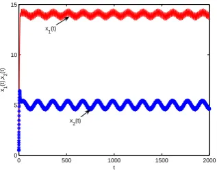
Example 4.1.Consider the following Nicholson-type system with time-varying delays
˙
x1(t) =−a1x1(t) +b1x2(t)
+c1(t)x1(t−τ)e−x1(t−τ),
˙
x2(t) =−a2x2(t) +b2x1(t)
+c2(t)x2(t−τ)e−x2(t−τ),
(22)
wherea1 = 5, a2 = 4, b1=−2, b2=−2, c1(t) =e2(0.5 +
0.5 sint), c2(t) =e2(0.4 + 0.6 cost), τ = 0.5. It is easy to
check that all the conditions (H1) and (H2) are satisfied. Thus system (22) has exactly one positive solution which is globally exponentially stable. The results are illustrated in Fig.1.
0 500 1000 1500 2000
0 5 10 15
t
x1
(t),x
2
(t)
x1(t)
x
[image:4.595.346.505.60.187.2]2(t)
Fig. 1. Transient response of state variablesx1(t)andx2(t).
0 500 1000 1500 2000
0 5 10 15
t
x1
(t),x
2
(t)
x1(t)
[image:4.595.50.291.61.369.2]x2(t)
Fig. 2. Transient response of state variablesx1(t)andx2(t).
Example 4.2.Consider the following Nicholson-type system with time-varying delays
˙
x1(t) =−a1x1(t) +b1x2(t)
+c1(t)x1(t−τ)e−x1(t−τ),
˙
x2(t) =−a2x2(t) +b2x1(t)
+c2(t)x2(t−τ)e−x2(t−τ),
(23)
wherea1= 6, a2= 5, b1 =−3, b2 =−3, c1(t) =e3(0.6 +
0.6 cost), c2(t) =e3(0.6 + 0.4 sint), τ = 0.3. It is easy to
check that all the conditions (H1) and (H2) are satisfied. Thus system (23) has exactly one positive solution which is globally exponentially stable. The results are illustrated in Fig. 2.
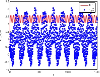
Example 4.3.Consider the following Nicholson-type system with time-varying delays
˙
x1(t) =−a1x1(t) +b1x2(t)
+c1(t)x1(t−τ)e−x1(t−τ),
˙
x2(t) =−a2x2(t) +b2x1(t)
+c2(t)x2(t−τ)e−x2(t−τ),
(24)
where a1 = 7.2, a2 = 6.1, b1 = −3.8, b2 = −2.5, c1(t) = e3(0.16 + 0.16 sint), c
2(t) =e4(0.16 + 0.12 sint), τ = 0.12.
It is easy to check that all the conditions (H1) and (H2) are satisfied. Thus system (24) has exactly one positive solution which is globally exponentially stable. The results are illustrated in Fig. 3.
Example 4.4.Consider the following Nicholson-type system
IAENG International Journal of Applied Mathematics, 45:2, IJAM_45_2_09
0 500 1000 1500 2000 −1
−0.5 0 0.5 1 1.5 2 2.5 3 3.5
t
x1
(t),x
2
(t)
[image:5.595.87.247.61.186.2]x1(t) x2(t)
Fig. 3. Transient response of state variablesx1(t)andx2(t).
0 500 1000 1500
−1 −0.5 0 0.5 1 1.5 2 2.5 3 3.5
t
x1
(t),x
2
(t)
[image:5.595.346.503.62.187.2]x1(t) x2(t)
Fig. 4. Transient response of state variablesx1(t)andx2(t).
with time-varying delays
˙
x1(t) =−a1x1(t) +b1x2(t)
+c1(t)x1(t−τ)e−x1(t−τ),
˙
x2(t) =−a2x2(t) +b2x1(t)
+c2(t)x2(t−τ)e−x2(t−τ),
(25)
wherea1 = 6.23, a2= 5.78, b1=−2.45, b2 =−3, c1(t) = e5(0.77+0.77 sint), c
2(t) =e7(0.77+0.62 cost), τ = 0.72.
It is easy to check that all the conditions (H1) and (H2) are satisfied. Thus system (25) has exactly one positive solution which is globally exponentially stable. The results are illustrated in Fig. 4.
Example 4.5.Consider the following Nicholson-type system with time-varying delays
˙
x1(t) =−a1x1(t) +b1x2(t)
+c1(t)x1(t−τ)e−x1(t−τ),
˙
x2(t) =−a2x2(t) +b2x1(t)
+c2(t)x2(t−τ)e−x2(t−τ),
(26)
wherea1= 8, a2= 3, b1=−2, b2=−4, c1(t) =e5(0.38 +
0.38 sint), c2(t) =e5(0.38 + 0.44 cost), τ = 0.52.It is easy
[image:5.595.87.247.228.352.2]to check that all the conditions (H1) and (H2) are satisfied. Thus system (26) has exactly one positive solution which is globally exponentially stable. The results are illustrated in Fig. 5.
Example 4.6.Consider the following Nicholson-type system with time-varying delays
˙
x1(t) =−a1x1(t) +b1x2(t)
+c1(t)x1(t−τ)e−x1(t−τ),
˙
x2(t) =−a2x2(t) +b2x1(t)
+c2(t)x2(t−τ)e−x2(t−τ),
(27)
0 500 1000 1500
−1 0 1 2 3 4 5
t
x1
(t),x
2
(t)
x1(t) x2(t)
Fig. 5. Transient response of state variablesx1(t)andx2(t).
0 500 1000 1500
−4 −2 0 2 4 6 8 10 12 14
t
x1
(t),x
2
(t)
x1(t) x2(t)
Fig. 6. Transient response of state variablesx1(t)andx2(t).
wherea1= 8, a2= 3, b1=−4, b2=−6, c1(t) =e5(0.76 +
0.76 cost), c2(t) =e4(0.76 + 0.67 sint), τ = 0.02.It is easy
to check that all the conditions (H1) and (H2) are satisfied. Thus system (27) has exactly one positive solution which is globally exponentially stable. The results are illustrated in Fig. 6.
Example 4.7.Consider the following Nicholson-type system with time-varying delays
˙
x1(t) =−a1x1(t) +b1x2(t)
+c1(t)x1(t−τ)e−x1(t−τ),
˙
x2(t) =−a2x2(t) +b2x1(t)
+c2(t)x2(t−τ)e−x2(t−τ),
(28)
wherea1= 4, a2= 3, b1=−2.6, b2=−4, c1(t) =e2(0.2+
0.2 cost), c2(t) =e4(0.5 + 0.1 sint), τ = 0.29.It is easy to
check that all the conditions (H1) and (H2) are satisfied. Thus system (28) has exactly one positive solution which is globally exponentially stable. The results are illustrated in Fig. 7.
Example 4.8.Consider the following Nicholson-type system with time-varying delays
˙
x1(t) =−a1x1(t) +b1x2(t)
+c1(t)x1(t−τ)e−x1(t−τ),
˙
x2(t) =−a2x2(t) +b2x1(t)
+c2(t)x2(t−τ)e−x2(t−τ),
(29)
where a1 = 5.002, a2 = 4.902, b1 = −2.305, b2 =
−3.002, c1(t) = e2(0.6012 + 0.6012 cost), c2(t) = e2(0.6012+0.3 sint), τ = 0.3.It is easy to check that all the
conditions (H1) and (H2) are satisfied. Thus system (29) has
IAENG International Journal of Applied Mathematics, 45:2, IJAM_45_2_09
[image:5.595.347.502.230.356.2]0 500 1000 1500 −2
0 2 4 6 8 10
t
x1
(t),x
2
(t)
[image:6.595.89.244.62.186.2]x1(t) x2(t)
Fig. 7. Transient response of state variablesx1(t)andx2(t).
0 500 1000 1500
0 5 10 15 20 25 30 35 40 45
t
x1
(t),x
2
(t)
x1(t) x
[image:6.595.90.246.233.359.2]2(t)
Fig. 8. Transient response of state variablesx1(t)andx2(t).
0 500 1000 1500
−20 −15 −10 −5 0 5 10 15
t
x1
(t),x
2
(t)
x
1(t)
x2(t)
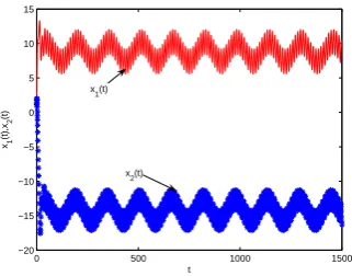
Fig. 9. Transient response of state variablesx1(t)andx2(t).
exactly one positive solution which is globally exponentially stable. The results are illustrated in Fig. 8.
Example 4.9.Consider the following Nicholson-type system with time-varying delays
˙
x1(t) =−a1x1(t) +b1x2(t)
+c1(t)x1(t−τ)e−x1(t−τ),
˙
x2(t) =−a2x2(t) +b2x1(t)
+c2(t)x2(t−τ)e−x2(t−τ),
(30)
where a1 = 5.7, a2 = 3.9, b1 =−2.9, b2 =−2.98, c1(t) = e4(0.2 + 0.2 sint), c
2(t) = e2(0.75 + 0.35 sint), τ = 0.21.
It is easy to check that all the conditions (H1) and (H2) are satisfied. Thus system (30) has exactly one positive solution which is globally exponentially stable. The results are illustrated in Fig. 9.
V. CONCLUSIONS
In this paper, we investigated a class of Nicholson-type sys-tem with delays. Applying the fundamental solution matrix, inequality techniques, Lyapunov function and constructing fundamental function sequences, some sufficient conditions which ensure the boundedness and exponential stability of positive solutions of Nicholson-type delay system are established. The obtained conditions are easily checked in practice by simple algebraic methods. Our results are new and supplement some previously known ones. Recently, Nicholson-type delay system with stochastic perturbation have also paid more attention by many scholars. However, there are rare results on the stability of solutions of stochastic Nicholson-type delay system, which might be our future research topic.
ACKNOWLEDGMENT
The authors would like to thank the anonymous referees for their helpful comments and valuable suggestions, which led to the improvement of the manuscript.
REFERENCES
[1] A. Nicholson, “An outline of the dynamics of animal populations,”
Australian Journal of Zoology, vol. 2, pp. 9-65, 1954.
[2] W. Gurney, S. Blythe, and R. Nisbet, “Nicholson,s blowflies revisited,”
Nature, vol. 287, pp. 17-21, 1980.
[3] R. Nisbet, and W. Gurney, Modelling Fluctuating Populations, John Wiley and Sons, NY, 1982.
[4] L. Berezansky, E. Braverman, and L. Idels, “Nicholson,s blowflies
differential equations revised: main results and open problems,”Applied Mathematical Modelling, vol. 34, pp. 1405-1417, 2010.
[5] J.O. Alzabut, “Almost periodic solutions for an impulsive delay Nicholson,s blowflies model,” Journal of Computational and Applied
Mathematics, vol. 234, no. 1, pp. 233-239, 2010.
[6] H.S. Ding, and J.J. Nieto, “A new approach for positive almost solutions to a class of Nicholson,s blowflies model,”Journal of Computational
and Applied Mathematics, vol. 253, pp. 249-254, 2013.
[7] L. Duan, and L.H. Huang, “Pseudo almost periodic dynamics of delay Nicholson,s blowflies model with a linear harvesting term,”
Mathematical Methods in the Applied Sciecnes, vol. 38, no. 6, pp: 1178C1189, 2015.
[8] W. Chen, and B. Liu, “Positive almost periodic solution for a class of Nicholson,s blowflies model with multiple time-varying delays,”
Journal of Computational and Applied Mathematics, vol. 235, no. 8, pp. 2090-2097, 2011.
[9] B.W. Liu, “The existence and uniqueness of positive periodic solutions of Nicholson-type delay system,” Nonlinear Analysis: Real World Applications, vol. 12, no. 6, pp. 3145-3151, 2011.
[10] Y. Chen, “Periodic solutions of delayed periodic Nicholson,s blowflies
model,”Canadian Applied Mathematics Quarterly, vol. 11, pp. 1838-1844, 2003.
[11] S. Saker, and S. Agarwal, “Oscillation and global attractivity in a periodic Nicholson,s blowflies model,”Mathematical and Computer
Modelling, vol. 35, no. 7-8, pp. 719-731, 2002.
[12] J.W. Li, and C.X. Du, “Existence of positive periodic solutions for a generalized Nicholson,s blowflies model,”Journal of Computational
and Applied Mathematics, vol. 221, no. 1, pp. 226-233, 2008. [13] L. Berezansky, L. Idels, and L. Troib, Global dynamics of
Nicholson-type delay systems with applications, Nonlinear Anal.: Real World Applications, vol. 12, no. 1, pp. 436-445, 2011.
[14] W. Wang, L. Wang, W. Chen, “Existence and exponential stability of positive almost periodic solution for Nicholson-type delay systems,”
Nonlinear Analysis: Real World Applications, vol. 12, no. 4, pp. 1938-1949, 2011.
[15] L. Berezansky, E. Braverman, and L. Idels, “Nicholson,s blowflies
differential equations revised: main results and open problem,”Applied Mathematcal Modelling, vol. 34, no. 6, pp. 1405-1417, 2010. [16] X.G. Liu, and J.X. Meng, “The positive almost periodic solution for
Nicholson-type delay systems with linear harvesting terms,” Applied Mathematical Modelling, vol. 36, no. 7, pp. 3289-3298, 2012.
IAENG International Journal of Applied Mathematics, 45:2, IJAM_45_2_09
[image:6.595.86.247.404.530.2][17] T. Faria, “Global asymptotic behaviour for a Nicholson model with path structure and multiple delays,”Nonlinear Analysis, vol. 74, no. 18, pp. 7033-7046, 2011.
[18] L.V. Hien, “Global asymptotic behaviour of positive solutions to a non-autonomous Nicholson,s blowflies model with delays,”Journal of
Biological Dynamics, vol. 8, no. 1, pp. 135-144, 2014.
[19] P. Amster, and A. Deboli, “Existence of positiveT-periodic solutions of a generalized Nicholson,s blowflies model with a nonlinear
harvest-ing term,”Applied Mathematics Letters, vol. 25, no. 9, pp. 1203-1207, 2012.
[20] Q.Y. Zhou, “The positive periodic solution for Nicholson-type delay system with linear harvesting terms,”Applied Mathematical Modelling, vol. 37, no. 8, pp. 5581-5590, 2013.
[21] F. Long, “Positive almost periodic solution for a class of Nicholson,s
blowflies model with a linear harvesting term,” Nonlinear Analysis: Real World Applications, vol. 13, no. 2, pp. 686-693, 2012.
[22] R.P.G. Mendes, M.R.A. Calado, and S.J.P.S. Mariano, “Analysis of the influence of different topologies on a TLSRG generation performance for WEC,”Engineering Letters, vol. 22, no. 4, pp. 202-208, 2014. [23] S. Okamoto, and A. Ito, “Effect of nitrogen Atoms and grain
boundaries on shear properties of graphene by molecular dynamics simulations,”Engineering Letters, vol. 22, no. 3, pp. 142-148, 2014. [24] C. Abagnale, M. Cardone, P. Iodice, S. Strano, M. Terzo, G. Vorraro,
“Theoretical and experimental evaluation of a chain strength measure-ment system for pedelecs,”Engineering Letters, vol. 22, no. 3, pp. 102-108, 2014.
[25] X.B. Qian, “Control-limit policy of condition-based Maintenance optimization for multi-component system by means of monte carlo simulation,”IAENG International Journal of Computer Science, vol. 41, no. 4, pp. 269-273, 2014.
[26] D. Huynh, D. Tran, and W.L. Ma, “Contextual analysis for the representation of words,”IAENG International Journal of Computer Science, vol. 41, no. 2, pp. 148-152, 2014.
[27] C.J. Xu, Y.S. Wu, and L. Lu, “On Permanence and asymptotically periodic solution of a delayed three-level food chain model with Beddington-DeAngelis functional response,”IAENG International Jour-nal of Applied Mathematics, vol. 44, no. 4, pp. 163-169, 2014. [28] F. Hosseini Shekarabi, M. Khodabin, and K. Maleknejad, The
petrov-galerkin method for numerical solution of stochastic Volterra integral equations,IAENG International Journal of Applied Mathematics, vol. 44, no. 4, pp. 170-176, 2014.
[29] B.W. Liu, and S.H. Gong, “Permanence for Nicholson-type delay system with nonlinear density-dependent mortality terms,”Nonlinear Analysis: Real World Applications, vol. 12, no. 4, pp. 1931-1937, 2011. [30] L. Berezansky, L. Idels, and L. Troib, “Global dynamics of Nicholson-type delay system with applications,”Nonlinear Analysis: Real World Applications, vol. 12, no.1, vol. 436-445, 2011.
[31] L. Shilnikov, A. Shilnikov, D. Turaev, and L. Chua, Methods of qualitative Theory in Nonlinear Dynamics, Part I, World Scientific, Singapore, New Jersey, London, Hong Kong, 1999.