A Novel Combination Scheme for Rayleigh-Taylor Instability Problem in the Laser Ablation Simulation

(1)

A Novel Combination Scheme for Rayleigh-Taylor

Instability Problem in the Laser Ablation

Simulation

Cunyun Nie, Haizhuan Yuan, Yuyue Yang, and Shuanggui Li

Abstract—The laser ablation is one important part in the inertial confinement fusion (ICF) simulation. The Rayleigh-Taylor (R-T) instability problem is always described as the radiative fluid dynamics equations which are always character-istic of strong nonlinearity and severely discontinuous interface. It can usually be decoupled into radiative fluid dynamics and heat transfer parts with its essential properties. We present a numerical algorithm for the decoupled system. To realize this algorithm, we put forward a combined scheme which inherits some advantages of both FDWENO and RKDG for fluid equa-tions, and construct a symmetric bilinear finite volume element (SBLFVE) scheme for the heat transfer equation. Furthermore, to obtain the proper time step size, we design an adaptive algorithm to harmonize and balance the decoupled system, and to accelerate the computation. We carry on some numerical simulations. Numerical results reveal the bounce phenomena of the shock, the processes of breaking and splitting of thick layer CH, and symmetric temperature distributions, and also show that the reflect wave emerges on some boundary after the laser’s erosion. These results also validate the correctness and robustness of the schemes and algorithms.

Index Terms—Rayleigh-Taylor instability problem, decou-pling algorithm, combined scheme, bilinear finite volume el-ement scheme, adaptive algorithm.

I. INTRODUCTION

T

HE radiative fluid dynamics problem, such as iner-tial confinement fusion simulation, is attractive and challenging for many physics and mathematical researchers all along these years ([1], [2], [3], [4], [5]). To solve the Rayleigh-Taylor instability problem is one important part of inertial confinement fusion experiments, and there appeared many literatures discussing its numerical simulations ([6], [7], [8], [9], [10], [11], [12], [13]). Its characteristics is that the high density fluid with the shape like long spike of rice flows in the low density one, and is that the long spike fluid becomes the shape of mushroom after some periods, and is that the low density fluid is squeezed into the high density region. In ICF numerical experiments, the radiation fluid dynamics problem is described by some control partial differential equations for the laser-driven implosion of a fuel capsule with the goal of igniting a self-sustained reaction. In experiments, the Rayleigh-Taylor instability effects greatly on the inertial fusion, temperature, igniting and flame.

Manuscript received Sept. 22, 2018; revised Feb. 2, 2019. This work was supported by the Project of Scientific Research Fund of Hunan Provincial Education Department (Grant No. 14B044), and the Developing Foundation of CAEP (No. 2015B0202033).

Corresponding author. Cunyun Nie is with the School of Science, Hunan Institute of Engineering, Hunan, 411104, China. e-mail: [email protected]. Haizhuan Yuan and Yuyue Yang are with the School of Mathematical and Computational Science, Xiangtan University, Hunan, 411105, China.

Shuanggui Li is with the Institute of Applied Physical and Computational Mathematics, Beijing, 10094, China.

In this work, the radiative fluid dynamic problem is decoupled as radiative fluid dynamics and heat transfer parts with preserving its essential properties. Our first work is to design one efficient numerical algorithm for this decoupled system. The first step of it is to obtain a proper guess by solving this system with some explicit scheme. The second step is to renew the temperature and total energy by the state equation. Final step is to obtain the very temperature by solving the energy equation with some implicit scheme. The second work is to present a composite scheme composed of the fifth-order FDWENO and third-order RKDG schemes for fluid equations. It holds the advantages of above two schemes, where the relative function values at fictitious nodes can be provided for each other. We also construct a SBLFVE scheme for the heat transfer equation. The symmetry of it is helpful for numerical simulations. The third work is to put forward a time adaptive algorithm to harmonize the computations between the fluid dynamics and the heat transfer. It can ensure numerical simulation to be accelerative and stable. Numerical simulations are carried on. Numerical results reveal some physical phenomena: the bounce of the stock, the break and split process of thick layer of CH. Numerical results also show that the density has changed after the laser’s erosion in the high density region (CH target region), and show that the reflect wave emerges on left boundary at some time, and show that symmetric temperature distributions confirm the heat transfer process. These results validate the correctness and robustness of our novel scheme. The remainder of this paper is organized as follows. In Section II, we introduce the model problem. In Section III, we present the decoupled algorithm. In Section IV, we design two schemes for the decoupled system. Finally we display numerical results to support our schemes and algorithms.

II. THE BACKGROUND AND THE MODEL PROBLEM

The radiative fluid dynamics problem usually includes the mass, monument and energy conservative equations as follows

         

        

∂ρ

∂t+∇ ·(ρ~u) = 0, ∂(ρ~u)

∂t +∇ ·(ρ~u~u) +∇(Pe+Pi+Pr) = 0, ∂(ρEe)

∂t +∇ ·(ρEe~u+Pe~u) =∇ ·(Ke∇Te)

+ρWei(Ti−Te) +ρWer(Tr−Te), ∂(ρEi)

∂t +∇ ·(ρEi~u+Pi~u) =∇ ·(Ki∇Ti)

+ρWei(Te−Ti), ∂(ρEr)

∂t +∇ ·(ρEr~u+Pr~u) =∇ ·(Kr∇Tr)

+ρWer(Te−Tr),

(1)

where Tj, Pj, Kj, Ej and εj, j = e, i, r are the temperature,

pressure, heat transfer coefficient, total energy (for unit mass point)

IAENG International Journal of Applied Mathematics, 49:2, IJAM_49_2_13

(2)

and the ratio of inner energy of the electron, the ion and the photon, respectively, and~uis the velocity, and

Ej=εj+

1

2~u·~u, j=e, i, r, (2) and ρ is the density, and Wei, Wer are the energy exchange

coefficients between the electron and the ion, between the electron and the photon, respectively.

In Equation (1), the energy conservation law can be described by three temperature equations from the following relations

εj(ρ, Tj) = 1.5ΓjTj, j=e, i, εr(ρ, Tr) =

1

ρaT

4

r,

and there exist some expressions about above physics variables

Kj=AkjT

5/2

j , j =e, r, Kr= 0.3×107lrTr3,

lr=Arρn1Trn2, Wei=AeiρT −3/2

e , Wer=AerρT −1/2

e ,

Pj(ρ, Tj) = ΓjρTj, j=e, i, Pr(ρ, Tr) =1₃aTr4,

(3)

and here a is the size of the target ball, and Ake, Aki, Ar, n1,

n2,Aei,Aer,Γe,Γiare some given constants.

Equations (1) (2) and (3) can constitute a self-closed system for simulating the implosion procession, together with some computa-tion region, initial-value and boundary condicomputa-tions. To be convenient, we only consider the case of single temperature in one material region. In this case, it can be simplified as the following R-T instability problem

Ut+F(U)x+G(U)y=f, (x, y)∈Ω, (4)

where

U = (ρ, ρu, ρv, ρE)t,

F(U) = (ρu, ρu2+p, ρuv, u(ρE+p))t, G(U) = (ρv, ρvu, ρv2+p, v(ρE+p))t,

f= (0,0,0,∇ ·(K∇T) +Q)t, ρE=ρ+1

2ρ(u

2

+v2),

and state equations

p= (γ−1)ρ, ρE= p

γ−1+ρ(u

2

+v2)/2, p=RρT, =CvT =E−(u2+v2)/2.

In above equations

and E are the unit volume inner energy and total energy, respectively.

u and v are the velocity along the direction of x-axis , y-axis, respectively.

T is the temperature, andK is the heat transfer coefficient

K=

k1 0

0 k2

, ki=aiT5/2, i= 1,2,

a1=

p

1 +qT∂T ∂x/ρ

, a2=

p

1 +qT∂T ∂y/ρ

, pandqare some constants.

Q is the heat resource (the laser radiation), and R is the gas coefficient, andCvis the ratio of specific heat.

We will endow equation (4) with some suitable conditions.

(i) Computation region: a rectangle regionΩ =

3

S

i=1

[image:2.595.333.520.52.124.2]

Ωishown as

Fig. 1 where Ω1,Ω2 and Ω3 are the quadrilateral regions ABDC,

CDFE and EFHG, respectively.

(ii) Boundary conditions: outflow boundary onΓ4, wall reflection

boundary onΓi, i= 1,2,3.

(iii) Initial-value conditions: initial density, velocity and temper-ature at timet0 are as follows, respectively,

ρ0 =

( _ρ

1, (x, y)∈Ω1,

1.0 +δcos(250lπy/3), (x, y)∈Ω2,

ρ2, (x, y)∈Ω3,

(5)

Fig. 1. The computation region.

whereρ1, ρ2, δ, l, πare some given constants,

u0=v0= 0, T0= 3.0×10 −4

.

So far, R-T instability problem (4) is well-posed.

III. DECOUPLING ALGORITHM

Numerical simulations for R-T instability problem (4) are always challenging due to its strong nonlinearity and severely discontinu-ousity. It is usually difficult to solve it directly. Fortunately, it can be decoupled into one radiative fluid dynamics equation and one radiative heat transfer equation as follows

Ut+F(U)x+G(U)y= 0, (x, y)∈Ω, (6)

ρCv

∂T ∂t =

∂ ∂x(K1

∂T ∂x) +

∂ ∂y(K2

∂T

∂y) +Q, (x, y)∈Ω, (7)

where initial and boundary conditions are the same as those before decoupled.

Firstly, we can take the partition for the time interval[0, te]

0 =t0< t1< t2 <· · ·< tN=te, (8)

and denote∆tn=tn+1−tn, n= 0,· · ·, N−1.

Assuming that all variable values at timetnare given, we need

find those at timetn+1. We will design some numerical algorithms

for Equations (6) and (7) in the following.

Algorithm 1:

Step 1: compute the parametersa1, a2 at timetn, and obtain

the variable valuesρn+1, un+1, vn+1, E¯at timetn+1by solving

Equation (6), whereE¯is a transition variable. Step 2: computeT¯according to the state equation

cvT¯= ¯E−((un+1)2+ (vn+1)2)/2.

Step 3: obtain the temperatureTn+1 at timetn+1 by solving

Equation (7) whereT¯and ρn+1 are treated as the values at time

tn.

Step 4: compute the new energyEn+1at timetn+1

En+1=cvTn+1+ ((un+1)2+ (vn+1)2)/2.

By above4steps, we can obtain all variable values at timetn+1,

and finish one time step computation for Equation (4).

Remark 1:

(1) In Step 3, we firstly choose a proper time step size∆tn to

solve Equation (6). It will be forced to choose a smaller one and to resolve it if it doesn’t converge as solving Equation (7) by using ∆tn.

(2)The Courant Friedrichs condition should be also satisfied with. (3) The similar algorithm can be employed for other complex system.

IV. TWO SCHEMES FOR DECOUPLING ALGORITHM

We will introduce a combined scheme for Equation (6) and a SBLFVE scheme for Equation (7), respectively. On the scope of the author’s knowledge, there is not any literature on above two schemes composed and employed for the R-T instability problem.

IAENG International Journal of Applied Mathematics, 49:2, IJAM_49_2_13

(3)

A. The combined scheme

In this subsection, we will display a novel scheme combining the fifth-order FDWENO with third-order RKDG schemes for Equation (6).

We take the quadrilateral partition for RegionΩ, and denote it as Ωh = {Ei,1 ≤ i ≤ M}, where Ei is any element, and M

is the total number of elements. Simultaneously, we take the dual partition ofΩh, and denote it asΩh∗={bXk,1≤k≤N}, where

Xk= (xi, yj)is some partition node, andN is the total number

of nodes.

By the backward Euler method, Equation (6) becomes

Un+1₋_Un

∆tn

+F(Un+1)x+G(Un+1)y= 0,

where∆tn=tn+1−tn.

LetU =Un+1

, and we have

U−Un

∆tn

+F(U)x+G(U)y= 0.

The next task is to discretise the term (F(U(t, x, y))x)(i,j) +

(G(U(t, x, y))y)(i,j) ( Denoted asI(t, xi, yi)).

The first thing for this task is to discretize I(t, x, y) by the FDWENO scheme on uniform grids (∆x,∆yis the step size along the x-axis and y-axis direction, respectively ) at Point(xi, yj)where

numerical fluxes should satisfy with the Lipschitz and consistent conditions.

I(x, y, t)≈ 1

∆x( ˆFi+1/2,j−Fˆi−1/2,j)+

1

∆y( ˆGi,j+1/2−Gˆi,j−1/2),

(9) where

ˆ

Fi+1/2,j= ˆF

+

i+1/2,j+ ˆF − i+1/2,j,

ˆ

F_i±₊₁_/₂_,j=

k−1

X

r=0

ωrFˆ ± (r)

i+1/2,j, Fˆ ± i−1/2,j =

k−1

X

r=0

˜

ωrFˆ ± (r)

i−1/2,j,

ωr=

αr k−1

P

s=0

αs

,ω˜r=

˜

αr k−1

P

s=0

˜

αs

, αr=

dr

(ε+βr)2

,α˜r=

˜

dr

(ε+βr)2

,

and for the fifth-order FDWENO scheme, we choosek= 3,

β0=

13

12(Ui−2Ui+1+Ui+2)

2

+1

4(3Ui−4Ui+1+Ui+2)

2

, β1=

13

12(Ui−1−2Ui+Ui+1)

2

+1

4(Ui−1−Ui+1)

2

, β2=

13

12(Ui−2−2Ui−1+Ui)

2

+1

4(Ui−2−4Ui−1+ 3Ui)

2

. d0=

3 10, d1=

3 5, d2=

1 10,

˜

dr=d2−r, r= 0,1,2,

andε= 10−6 or10−12, ˆ

F_i−₊₁(_/r₂)_,j=

k−1

X

r=0

crjF − i−r+j,Fˆ

+ (r)

i−1/2,j= k−1

X

r=0

˜

crjFi+−r+j,

andcij is shown as Tab. 1, and ˜crj=cr−1,j, r=0,1,2,

and Gˆi,j+1/2= ˆG+i,j+1/2+ ˆG −

i,j+1/2 can be similarly presented.

Above choices can helpfully guarantee to solve Equation (6) which inherits both strong discontinuousity and great density ratio. The forgoing thing for this task is to discretizeF(U)x+G(U)y

by the third-order RKDG scheme on rectangle grids.

For any element Ek (also denoted by Ei,j), from the Green

formula,

I(t, x, y) = (10) X

e∈∂Ei,j

Z

e

(F(Uh(t,x)), G(Uh(t,x)))·ne,Ei,jvh(x)dΓ

−

Z

Ei,j

F(Uh(t,x))

∂vh(x)

∂x +G(Uh(t,x)) ∂vh(x)

∂y

dx,

TABLE I THE COEFFICIENTScr,j.

k r j= 0 j= 1 j= 2

−1 1

1 0 1

−1 3₂ −1 2

2 0 1₂ 1₂ 1 −1

2 3 2

−1 11₆ −7 6

1 3

3 0 1₃ 5₆ −1 6

1 −1₆ 5₆ 1₃

2 1₃ −7 6

11 6

wherex= (x, y), andvh(x)can be usually chosen as some kind

of orthogonal basis functionφi,j(x, y), such as

1, αi(x) =

x−xj

∆xh/2

, βj(y) =

y−yj

∆yh/2

, αi(x)βj(y),

α2i(x)−

1 3, β

2

j(y)−

1 3. Substituting φi,j(x) into vh in (10) and employing Gaussian

integral formula,

I(t, x, y)≈ L

X

l=1

ωlV1F,G·ne,Ei,jφi,j(xe,l)|e|

− M

X

m=1

˜

ωmV2F,G· ∇φi,j(x)|Ei,j|,

where

V1F,G= (F(Uh(t,xe,l)), G(Uh(t,xe,l))), V2F,G= F(Uh(t,xEi,j,m)), G(Uh(t,xEi,j,m))

,

and

(1)ωlandω˜mare the weights,xe,landxEi,j,m are the Gaussian points on Edgeeand in ElementEi,j, respectively,

(2)ne,Ei,j is the unit outward normal vector, and|e|,|Ei,j|is the

length of the edgee, the area of ElementEi,j, respectively,

(3)F(Uh(t,xEi,j,m)), G(Uh(t,xEi,j,m)can be approximated by

some numerical fluxes, such as the Local Lax-Fridrichs splitting. The final thing for this task is to combine above two schemes. The values at fictitious nodes for FDWENO scheme can be eval-uated by the polynomial in some element from RKDG scheme, and the data of fictitious element for RKDG scheme can be reconstructed by those from the forward time step of FDWENO scheme.

So far, the combined scheme has been designed to solve Equation (6).

B. Bilinear finite volume element scheme

By the backward Euler method, Equation (7) leads to

ρCvT−∆tn(

∂ ∂x(K1

∂T ∂x) +

∂ ∂y(K2

∂T

∂y)) (11)

= ∆tnQ+ρCvTn,

whereT :=Tn+1₌_T₍_t

n+1),Tn=T(tn),

Kl=Kl(T), l= 1,2.

According to the “fixed-coefficient” method, we can obtain

ρCvT−∆tn(

∂ ∂x(K

(k) 1

∂T ∂x) +

∂ ∂y(K

(k) 2

∂T

∂y)) (12)

= ∆tnQ+ρCvTn,

whereT :=T(k+1)₍_t

n+1)andT(k)=T(k)(tn+1)are the

approx-imations at the current and forward iterative steps, respectively, and

K_l(k)=Kl(T(k)).

IAENG International Journal of Applied Mathematics, 49:2, IJAM_49_2_13

(4)

We will construct a symmetrical bilinear finite volume element scheme for Equation (12) (Seen in [14], [15], [16], [17], [18]).

The finite element spaceVhis introduced as follows

Vh={uh∈C( ¯Ω) :uh|E=ϕEˆ◦ψ −1

E , ϕEˆ ∈ ∧P1,1, E∈Ωh,

uh|∂Ω= 0},

wherePˆ1,1 is the set of bilinear functions defined on the standard

elementEˆ, andϕEˆ◦ψ −1

E represents the composite function between

ϕEˆ(ˆx1,xˆ2) and ψ−E1, and here ψ −1

E is the inverse transformation

ofψE, and the bilinear transformation is fromEˆ toE.

Integrating (12) on the dual elementbXi∈Ω

h

∗, we have

Z

b_Xi

ρCvT dx−∆tn

Z

b_Xi

( ∂

∂x(K

(k) 1

∂T ∂x) +

∂ ∂y(K

(k) 2

∂T ∂y))dx

= Z

b_Xi

(∆tnQ+ρCvTn)dx.

By the Green formula, we can obtain

Z

b_Xi

ρCvT dx−∆tn

Z

∂b_Xi

(K1(k)

∂T ∂x, K

(k) 2

∂T

∂y)·nds (13)

= Z

b_Xi

(∆tnQ+ρCvTn)dx,

wherenis the unit outer normal vector.

ApproximatedT byTh∈Vhin (13), the balance equation leads

to Z

b_Xi

ρCvThdx−∆tn

Z

∂b_Xi

(K₁(k)∂Th ∂x , K

(k) 2

∂Th

∂y )·nds (14)

= Z

b_Xi

(∆tnQ+ρCvThn)dx.

One can see that

Th=

4

X

k=1

Th,kφk,

whereTh,k=Th(Xk),1≤k≤4, andXk, φkis the node, bilinear

Lagrange interpolation basis function on elementE, respectively. From Equation (14) and above expression of Th, one can also

obtain the element stiff matrix AE = (aEij)4×4 and element load

vectorfE = (fiE)4×1, where

aEij=

Z

Di

ρCvdxδij−∆tn

Z

∂Di

(K1(k)

∂φj

∂x, K

(k) 2

∂φj

∂y )|O·nds,

1≤i, j≤4, fiE=

Z

Di

(∆tnQ+ρCvThn)dx, 1≤i≤4,

and here δij =

1, i=j,

0, i6=j, , and O is the center of element

E, andDi, 1≤i≤4is the sub-control volume about NodeXi,

respectively.

Assembling all element stiff matrices and load vectors, and dealing with boundary conditions, we can obtain a symmetric bilinear finite volume element (SBLFVE) scheme for Equation (7).

C. Two schemes’ harmonization

We have obtained a combined scheme and a SBLFVE scheme for the decoupled system: Equations (6) and (7), respectively. It is important for them to choose a proper and common time step size ∆tn. Firstly, the CFL condition should be satisfied with. Secondly,

it is also vital to harmonize and balance two parts’ computations (radiative fluid mechanics and radiative heat transfer). In order to reach it, we design an adaptive algorithm as follows.

Algorithm 2:

Step 1: compute the inner energy at the current and forward time steps (denoted as(i,j) andn(i,j) ) for ElementEi,j, respectively.

Step 2: compute the change ratio of the inner energy for all elements

r(i,j)=|(i,j)−n(i,j)|/(i,j),

and find the maximumrmax= max i,j {ri,j}.

Step 3: determine the adjusted time step size according to the

rmax for some given change ratio r, such as 0.1, we design the

following three cases:

(1)The time step size preservesrifrmaxis close tor, i.e.r/2≤

rmax≤2r;

(2)The time step size becomes smaller thanr, such as 0.8 times

r, ifrmaxis more than2r;

(3)The time step size becomes bigger thanr, such as 1.25 times

r, ifrmaxis less thanr/2.

Step 4: in addition, we need also adjust the time step size according to the convergence of the nonlinear iteration, for some given maximum iteration numberN0(Usually chosen as 40), if the

real nonlinear iteration numberN > N0, the time step size should

become smaller, such as0.8r.

V. NUMERICAL EXPERIMENTS

In this section, we take numerical experiments for two types of R-T unstable problems driven by the gravity force and the laser, respectively.

Example 1(Seen in [9]) U = (0,0, ρg, ρgv)T_{, computation region}

Ω = [0,0.25]×[0,1]. The initial interface is the liney= 0.5, and the region wherey >0.5corresponds to the light fluid, other region does the weight one, and the gravitational accelerationgis along the y-axis direction.

Boundary conditions:

Left and right : wall boundary, Above:ρ= 1,u=v= 0, p= 2.5, Below:ρ= 2, u=v= 0, p= 1.

Initial conditions:

weight fluid:ρ= 2, u= 0, v=−0.025ccos(8πx), p= 2y+ 1, light fluid:ρ= 1, u= 0, v=−0.025ccos(8πx), p=y+3

2,

wherec=pγp

ρ is the speed of sound, andγ= 5/3,g= 1.

We carry on some numerical tests for the fifth-order FDWENO scheme and the combined scheme, where the uniform partition for the region Ω is Nx ×Ny = 60×240, and for the combined

scheme: Regionsy < y0andy≥y0are employed by the fifth-order

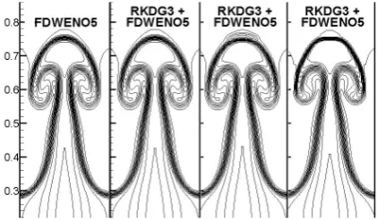
[image:4.595.320.531.535.658.2]

FDWENO, third-order RKDG schemes, respectively. We obtain the results at timet= 1.95 shown as Fig. 2 , where the first one is for the fifth-order FDWENO scheme, and others (from the second one to the fourth one) are for the combined scheme with different interfaces y0= 0.8, y0= 0.75,y0= 0.6, respectively.

Fig. 2. R-T unstable problem: the fifth-order FDWENO scheme (the first one) and a combined scheme with different interfaces y0 = 0.8,y0 =

0.75,y0= 0.6(the second one to the fourth one ), respectively.

From above results, one can see that they agree with those in the literature [9] when the interface is far from the discontinuous part, and the accuracy of the results becomes not very well but acceptable. The advantage of this combined scheme is that it can dispose with the composite discontinuous region efficiently.

In the following example, we carry on some numerical tests for the laser-driven Rayleigh-Taylor (R-T) instability problem (4) and realize Algorithms 1 and 2 by two ways: (1) the fifth-order

IAENG International Journal of Applied Mathematics, 49:2, IJAM_49_2_13

(5)

FDWENO scheme and the SBLFVE scheme, (2) the combined scheme and the SBLFVE scheme, respectively.

Example 2 For Model problem (4), we choose the parameters as follows.

The computation regionΩ(unit:µm)

AC= 0.1, CE= 0.01, EG= 1, AB= 0.024,

and for initial-value conditions

ρ1= 0.08, ρ2= 10 −3

, δ= 0.5, l= 1.

Some other parameters are as follows

R= 57.55, Cv= 86.325, γ= 5/3,

k1=a1T5/2, k2=a2T5/2,

a1=

p

1 +qT∂T ∂x/ρ

, a2=

p

1 +qT∂T ∂y/ρ

,

p= 0.00993957, q=0.18494×2 0.3243 ×10

−6

.

In the region where 0.1108 ≤ x ≤ 0.1268, the laser radiation resourceQsatisfies with

Q=

₃

1610

9_{t, t}_≤₀_.₀₀₁_, 3

1610

6_{, t >}₀_.₀₀₁_. (15)

In this example, we take the uniform partition for Region Ω:

Nx×Ny= 317×60, and the mesh size is4×10−4. The first

[image:5.595.320.535.53.188.2] [image:5.595.45.279.62.315.2]

and second ways are carried on. Numerical results for the first way are shown as Fig. 3 and Fig. 4, and those for the second way are shown as Fig. 5 and Fig. 6 . These results agree with those in the literature [10].

[image:5.595.307.547.216.309.2]

Fig. 3. The density contour for the way (1) FDWENO-SBLFVE scheme.

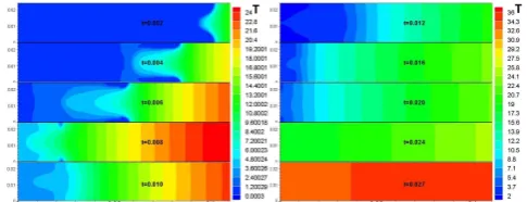
Fig. 4. Temperature distributions for the way (1) FDWENO-SBLFVE scheme.

Fig. 3 shows eight different contours at the corresponding time, respectively. Each of them reports that the bounce phenomena of the stock, the break and split process of thick layer of CH. The density has changed after the laser’s erosion in the high density region (CH target region). It also presents that the reflect wave emerges on left boundary at timet= 0.0064. Fig. 5 shows similar phenomena.

[image:5.595.61.279.387.522.2]

Fig. 4 displays some temperature distributions at different time. It presents good symmetry property, which confirms that the heat transfer is normal. Fig. 6 shows similar phenomena.

Fig. 5. The density contour for the way (2) conbined-SBLFVE scheme.

Fig. 6. Temperature distributions for the way (2) conbined-SBLFVE scheme.

We can pay attention to the fact that the flection wave on left boundary makes the convection dominate due to the outmost shell’s splitting. It leads to the temperature to become a bit lower locally. However, it increases quickly after that time, and reaches the maximum 36MK at timet= 0.027.

Numerical results validate the decoupling algorithm and two schemes for the decoupled system. It can provide some references for simulations of ICF problem.

VI. CONCLUSION

In this paper, the Rayleigh-Taylor instability problem is decoupled into radiative fluid dynamics and heat transfer parts. We put forward a combined scheme which inherits some advantages of both FDWENO and RKDG for fluid equations, and construct a symmetric bilinear finite volume element scheme for the heat transfer equation, and design an adaptive algorithm to harmonize the decoupled system. Numerical results reveal the bounce phenomena of the shock, the processes of breaking and splitting of thick layer CH, the symmetric temperature distributions, and the reflect wave emerging on some boundary after the laser’s erosion. These results confirm the validity of the schemes and algorithms.

ACKNOWLEDGEMENT

The authors thank the referees for their valuable suggestions to improve this paper greatly and are grateful to Professor Shi Shu and Doctor Chunsheng Feng for some helpful discussions on numerical experiments.

REFERENCES

[1] P. L. Roe, “Approximate riemann solvers, parameter vectors and differ-ence schemes,”Journal of Computational Physics, vol. 43, pp357-372, 1981.

[2] P. D. Lax, X. D. Liu, “Solution of two-dimensional Riemann problems of gas dynamics by positive schemes,” SIAM Journal of Scientific Computing, vol. 19, no. 2, pp319-340, 1998.

[3] O. Friedrichs, “Weighted essentially non-oscillatory schemes for the interpolation of mean values on unstructred grids,”Journal of Compu-tational Physics, vol. 144, pp194-212, 1998.

[4] Y. Ren, M. Liu, H. A. Zhang, “Characteristic-wise hybrid compact-WENO schemes for solving hyperbolic conservations,” Journal of Computational Physics, vol. 192, pp365-386, 2005.

IAENG International Journal of Applied Mathematics, 49:2, IJAM_49_2_13

[image:5.595.46.289.562.655.2]

(6)

[5] Ch. Yan, J. X. Yu and etc, “On the achievements and prospects for the methods of computational fluid dynamics,”Advances in mechanics, vol. 41, no. 5, pp562-589, 2011.

[6] J. Yang, N. Zhao, W. J. Tang, “Fiction fluid methods for nonstable interface numerical simulation,” Chinese Journal of Computational physics, vol. 20, no. 6, pp549-555, 2003.

[7] J. Glimm, J. Grove and etc, “The dynamics of bubble growth for Rayleigh-Taylor unstable interface,”Physics of Fluids, vol. 31, pp447-465, 1988.

[8] W. H. Ye, W. Y. Zhang, G. G. Chen, “Numerical simulation for the laser Rayleigh-Taylor unstable problem,”High power laser and particle beams, vol. 10, no. 3, pp403-408, 1998.

[9] S. Jing, Y. T. Zhang, C. W. Shu, “Resolution of high order WENO schemes for complicated flow structures,”Journal of Computational physics, vol. 186, pp690-696, 2003.

[10] S. F. Li, W. H. Ye and etc, “High order FD-WENO scheme for Rayleigh-Taylor unstable problem,”Chinese Journal of Computational physics, vol. 25, no. 4, pp379-386, 2008.

[11] J. F. Wu, W. Y. Miao and etc, “Experimantal analysis of indirective-drive ablative Rayleigh-Taylor unstability on Shenguang II,” High power laser and particle beams, vol. 27, no. 3, pp1-8, 2015. [12] A. N. Kashif, Z. A. Aziz and etc, “Convective heat transfer in

the boundary layer flow of a Maxwell fluid over a flat plate using an approximation technique in the presence of pressure gradient,”

Engineering Letters, vol. 26, no. 1, pp14-22, 2017.

[13] N. Dunna, A. Ramu and D. K. Satpathi, “Numerical solution to strong cylindrical shock wave in the presence of magnetic field,”Proceedings of the World Congress on Engineering2018, pp33-38.

[14] S. Shu, H. Y. Yu, Y. Q. Huang and C. Y. Nie, “A preserving-symmetry finite volume scheme and superconvergence on quadrangle grids,”International Journal of Numerical Analysis and Modeling, vol. 3, no. 3, pp348-360, 2006.

[15] C. Y. Nie, S. Shu, H. Y. Yu and J. Wu, “Superconvergence and Asymptotic Expansions for Bilinear Finite Volume Element Approx-imations,” Numerical Mathematics: Theory, Method and Appplication, vol. 6, pp408-423, 2013.

[16] C. Y. Nie, S. Shu, H. Y. Yu and Y. Y. Yang, “Superconvergence and Asymptotic Expansion for Semidiscrete Bilinear Finite Volume Element Approximation of the Parabolic Problem,”Computer and Mathematics with Applications, vol. 66, pp91-104, 2013.

[17] C. Y. Nie, H. Y. Yu, “A Novel Finite Volume Scheme with Geomet-ric Average Method for Radiative Heat Transfer Problems,” Applied Physics Frontier, vol. 1, no. 4, pp32-44, 2013.

[18] J. L. Yan and L. H. Zheng, “Linear conservative finite volume element schemes for the gardner equation,”IAENG International Journal of Applied Mathematics, vol. 48, no. 4, pp434-443, 2018.