Dynamical exchange interaction from time dependent spin density functional theory

Dynamical exchange interaction from time-dependent spin density functional theory

Maria Stamenova*and Stefano Sanvito School of Physics, Trinity College, Dublin 2, Ireland (Received 14 June 2013; published 25 September 2013)

We report onab initiotime-dependent spin-dynamics simulations for a two-center magnetic molecular complex within the framework of the time-dependent noncollinear spin-density functional theory. In particular, we discuss how the dynamical behavior of theab initiospin-density in the time domain can be mapped onto a model Hamiltonian based on the classical Heisenberg spin-spin interactionJS1·S2. By analyzing individual

localized-spin trajectories, extracted from the localized-spin-density evolution, we demonstrate a practical method for evaluating the effective Heisenberg exchange coupling constantJfrom first-principles simulations. We find thatJ, extracted in such a dynamical way, agrees quantitatively with that calculated by the standard density functional theory broken-symmetry scheme.

DOI:10.1103/PhysRevB.88.104423 PACS number(s): 75.30.Et, 31.15.ee, 75.10.Hk, 36.40.Cg

I. INTRODUCTION

In magnetic recording the typical time scale for magne-tization reversal is in the nanosecond range, and it is now believed that the ultimate limit for magnetization switching by magnetic field pulses may approach the picosecond mark.1

Down to the picosecond scale, the exchange interaction is constant in time and so is the magnetic anisotropy. This allows the dynamics of magnetization to be modeled in terms of the continuous Landau-Lifshitz-Gilbert equation,2_{usually solved}

with micromagnetic techniques.3 _{The spatial resolution of}

such techniques is chosen in view of the problem at hand and numerical considerations, but the equation of motion is always the same. At the most finely resolved and microscopic end of the modeling spectrum there are atomistic spin models,4

which have been proved to be a powerful tool for approaching the extreme phenomenology of the ultrafast magnetization dynamics.5,6 _{In these one associates individual classical spin}

vectors Si to all magnetic atoms, which are then coupled

through a time-independent Heisenberg Hamiltonian,

H = −

i>j

JijSi·Sj, (1)

whereJij are the pairwise Heisenberg exchange parameters.

The state of the art for the theory is then represented by performing atomistic dynamical simulations in which the Heisenberg Hamiltonian is completed by additional terms to include the spin-orbit interaction (or effective anisotropy terms), the dipole-dipole interaction, and the interaction with an external magnetic field. In order to account for thermal fluctuations, stochastic fields are added to the internal magnetic field in the equations of motion,5–7in the spirit of the Langevin dynamics. The discretized stochastic Landau-Lifshitz-Gilbert equation has been used in earlier works, for instance, to model thermally assisted magnetic relaxation in classical spin chains.8

The parameters of the theory, the exchange integrals and the anisotropy, are usually fitted to experiments or calculated from static density functional theory (DFT).7 _{In this second}

case usually the exchange is obtained with the so-called broken-symmetryapproach, proposed first by Noodleman.9_In

its DFT variant broken symmetry refers to an unrestricted-spin calculation for open-shell complexes, where opposite spin

densities are allowed to localize at different atomic sites. This broken-symmetry or low spin (LS) state, unlike the state with the highest spin (HS), is not an eigenstate of the full spin operator (hence the name). The exchange parameters are then determined by the difference between the total energy, Eα

(α=LS, HS), of the two spin states,

Jij =f(Si,Sj)(ELS−EHS), (2)

where various formulations of the spin-dependent functionf are possible, depending on the choice of basis and level of localization, and whereSiis the expectation value of the spin

operator acting locally at the atomic sitei(see, for instance, Refs.10and11).

The first demonstration of laser-induced ultrafast demagnetization12 in transition metals, however, opened a new frontier, namely, the possibility of manipulating and controlling the magnetization with ultrashort intense laser pulses.13 _{Here one reaches the femtosecond time resolution,}

where both the exchange interaction and the anisotropy may become time-dependent. Most importantly, in this limit the approximation of associating a classical spin of constant magnitude to an atom may break down. It makes sense that at a time scale where the electronic degrees of freedom evolve in time in a nonadiabatic way (the local magnetic moment changes in time), spin dynamics needs to be addressed at the electronic level. Yet, in order to interpret the results in a simple and transparent way, it is desirable to be able to map the electronic time-dependent simulations onto classical atomistic models based on the Heisenberg Hamiltonian. How to perform such a mapping, and whether this is at all possible, is the subject of the present paper. In particular, we will discuss how the evolution in time of the spin density in time-dependent DFT15 _{(TD-DFT, or, to be more specific, its extension to}

noncollinear spin,16_{the TD-SDFT}17_{) simulations can be used}

to extract an effective spin dynamics, which in turn can be mapped onto a Heisenberg Hamiltonian. As a byproduct of such analysis we will be able to extract exchange parameters, whose values are quantitatively very close to those calculated with the broken-symmetry approach.

Heisenberg model for a diatomic molecule. This will be useful to interpret our TD-SDFT results. In the same section we will describe the general aspect of the TD-SDFT simulations and explain how to integrate the instantaneous electron density in order to map the TD-SDFT results onto the Heisenberg model. Then, in the following two sections, we will present results for both a stretched H2dimer and a hypothetical H-He-H trimer. These are qualitatively different systems with respect to the spin-spin interaction: while in H2the spins of the two H atoms are coupled via direct exchange, the exchange interaction in H-He-H is indirect, asuperexchange,14 _{mediated across the}

closed-shell He atom. Finally, we will conclude.

II. MAGNETIC DIMER: THEORETICAL ASPECTS A. Implementation of the TD-SDFT method

Ab initiospin dynamics is simulated in the time domain with the state-of-the-art TD-SDFT codeOCTOPUS.18_{This is an}

open-source (GPL) package capable of simulating excitations of molecules or clusters to custom-designed electromagnetic fields beyond the linear response regime, i.e., by the explicit time propagation of the TD Kohn-Sham equations in a basis-free real-space representation. OCTOPUS provides an ideal environment for examining fundamental processes in the time domain. As such, our starting point towards understandingab initiospin dynamics has to be through the simplest complexes of non-spin-singlet atoms. In fact, the simplest possible real system, for which the Heisenberg spin Hamiltonian of Eq.(1) was originally conceived, is the hydrogen molecule. In its ground state H2 is closed shell (diamagnetic), but in the stretched dissociating state local spins can be defined for each of the hydrogen atoms (e.g., in the broken-symmetry LS state, the electrons localized on the opposite protons have particular and opposite spin expectation value,s₁z_,2= ±1/2). Hence the stretched H2 provides the simplest physical realization of a molecular spin dimer.

In order to excite spin dynamics in collinear spin dimers, we have introduced a spatial inhomogeneity into the magnetic field pulses available in OCTOPUS. Thus, an inhomogeneous transverse magnetic field pulse of a few femtosecond duration is used to generate a spin misalignment in the dimer. In order to quantify such misalignment, we need a measure for the spin of overlapping atoms. Although the TD-SDFT spin-density distribution is well defined at every instant, the spin state (and the charge) of an individual atom in a molecule or solid is not an observable. This, of course, prevents us from rigorously mapping the TD-SDFT dynamics onto a classical Heisenberg model. In fact, computing expectation values of local spin operators (e.g.,S1ˆ ·S2ˆ ) fromab initio wave functions is not a trivial task,19_{and it has been recently}

shown that a continuum of valid definitions of the local spin operator ˆSi exists.20 In order to overcome such difficulty we

have implemented an intuitiverotating spinapproximation for decomposing the spatial spin-density distribution into atomic contributions, which is based on defining an appropriate linear transformation. The idea is to use the two extreme states, the HS and LS spin-density distributions, as reference points for decomposing the spin density of any given noncollinear spin state obtained through TD-SDFT evolution, assuming

that it is simply a result of rigid rotation in space of the spin density in certain continuous regions surrounding the atoms. We will demonstrate that such a method allows us to practically eliminate from the definition of the local spins the dependence on the particular spatial volume around the atom and that this can be done for a wide range of interatomic distances. This gives us the opportunity to define, with a unique criterion, the local spin dynamical trajectories, and thus to extract an effective exchange parameterJ for the spin dimer. Interestingly, the results agree quantitatively with those obtained by the broken-symmetry method.

All the TD-SDFT simulations are performed at the level of the adiabatic local spin-density approximation (ALSDA)21 with the modified parametrization of the correlation functional by Perdew and Zunger.22 _{The electron density and all the}

observables are represented over a dense real-space grid (with a spacing of 0.1 ˚A), and the entire simulation box is a paral-lelepiped of square cross section (typically with a 12- ˚A side) and a length (along the axis of the molecule) ranging between 20 ˚A and 30 ˚A, depending on the length of the molecule considered (in the dissociating limit). The time propagation of the Kohn-Sham equation is performed via the Crank-Nicolson (implicit midpoint) rule and the Lanczos approximation of the propagator is used, as implemented inOCTOPUS.23The typical time step used in the simulations is 0.004 fs.

We consider first a generic two-center magnetic molecular complex, a spin dimer, as illustrated in Fig. 1(a). The ground-state DFT calculation is initialized in either the HS or the LS collinear configuration. In order to generate spin noncollinearity, a spatially inhomogeneous external magnetic field pulseBext(r,t) is applied to the TD-SDFT Hamiltonian:24

ˆ

HKS(r,t)= N

i

−h¯2∇i2

2m −μBσˆi·Bs(ri,t)

×δ(r−ri)+vs(r,t), (3)

where the sum runs over all (N) electrons in the system, Bs=Bxc+Bext is the effective magnetic field for the

Kohn-Sham (KS) orbitals,σˆi is the electronic spin operator,

μB is the Bohr magneton, andvsis the Kohn-Sham effective

electrostatic potential. We have implemented Bext(r,t)= B0(r) exp[−(t−t0)2/τ_B2] with a Gaussian time dependence and a varianceτBtypically between 2 and 5 fs. This is applied

soon after the beginning of the time-dependent simulation [t₀is chosen such thatBext(t =0) is sufficiently close to zero so that the discontinuity in the potential introduced att =0 is negligibly small]. For the spatial dependence B0(r), we have experimented with a few simple continuous integrable functions and found that, as long as they are not symmetric with respect to the center of the molecule, there is little qualitative difference in the resulting spin dynamics. In other words, the sought outcome of spin noncollinearity in the electronic structure is readily obtainable for a wide range ofB0(r). In particular, we have found that there is no qualitative difference between a divergence-free solenoidal field, for instance,

B0(x,y,z)=B0e[−(x−x0)2/ξ2]

×[ex+(x−x0)y/ξ2ey+(x−x0)z/ξ2ez],

σ2

σ₁

S

S

S

Σ

x

after pulse

-1 -0.5 0 0.5 1

S

z/ hi

_

i=1

i=2

0 1 2 3 40

1 2 3 4

Δ

Etot

(meV)

0 0.02 0.04 0.06 0.08 0.1

(ϕ

− π) / π

0 2 4 6 8

t (fs) -1

-0.5 0 0.5 1

S

z/ hi

_

50 100 0 5 10

t (fs)

0 10 20 30 40 50

Δ

Etot

(meV)

0 0.1 0.2 0.3 0.4

(ϕ

− π) / π

(a)

(c)

(b)

x z

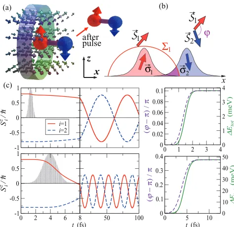
FIG. 1. (Color online) (a) Spin dynamics is excited by a transverse magnetic field pulse (as illustrated by the vector field schematic). The ring represents a hypothetical solenoid with its center lying on the bond axis (xaxis) and offset from the midpoint towards one of the atoms. (b) Illustration of the definition of local spinS1,2 [see

Eq.(11)] and the definition of the angleϕ. (c) Results from theab initiotime-dependent simulations for H2and two different durations

of the magnetic field pulse (shaded area): trajectories of the local spins’zcomponentSz

1,2, angleϕbetween them (broken purple line),

and the expectation value of the total TD-SDFT energy of the system (solid green line). The radius of the sphere definingS1,2isrsph=d/2

and the bond length isd=2.6 ˚A.

and the simplified B0(x,y,z)=B0exp[−(x−x0)2/ξ2]ex.

Hence, in most of the simulations we have used the latter, where (typically) x₀= −2 ˚A with respect to the center of the molecule,ξ =1 ˚A, andex is a unit vector along the x

axis (aligned with the spin-dimer axis). This corresponds to a magnetic field transverse to the direction of the initial (ground-state) spin polarization of the molecule, chosen as thezaxis [see Fig.1(a)]. We have used values ofB₀ranging from 0.5 to 10 kT in order to generate the desired misalignment for short enough simulation times. We note that these short, intense, and very localized magnetic field pulses are only to be taken as a tool for producing the misalignment, which onsets the spin dy-namics. They typically produce excitation of the system in the millielectronvolt range [see Fig.1(c), right-hand-side panels]. Below we analyze the classical version of this problem, i.e., the dynamics of two noncollinear classical angular momenta, S1andS2, interacting according to Eq.(1), and the possibility of mapping the TD-SDFT spin-density evolution onto that.

B. Classical Heisenberg model solution for a spin pair First, we examine the case of two rigid classical angular momenta S1,2 interacting according to a Heisenberg spin Hamiltonian:

Hcl= −2JclS1·S2. (5)

Since we choose to have|S1| = |S2| =S=1/2, the factor 2 in Eq.(5)is introduced in order forHclto produce the same difference between the energies of the parallel and antiparallel alignment of the classical spin pair as the triplet-singlet energy difference (or, equivalently, the broken-symmetry result for spin 1/2),

EBS= ↑↑|Hˆ|↑↑ − ↑↓|Hˆ|↑↓

=EHS−ELS= −J, (6)

for the corresponding quantum spin Hamiltonian

ˆ

H = −JS1ˆ ·S2ˆ . (7)

In the classical spin Hamiltonian [Eq. (5)] we include the physical dimension of the angular momenta (¯h) in the coupling constantJcl, which has a dimension of energy in analogy to

the exchange parameter J. Hence, the classical equation of motion for each spin, sayS1, is

˙

S1= {S1,Hcl}

= −2Jcl

l

S₂lS1,S₁l

= 2Jcl ¯

h S1×S2, (8)

where we have used the Poisson bracket for the corresponding classical angular momenta {Sk_h,S¯ m_{¯h} =ε}

klmSmh¯, with εklm

representing the fully antisymmetric Levi-Civita tensor. For classical spins, forming an arbitrary angleϕ, Eq.(8)describes a precessional motion about the total spin,Stot≡S1+S2, with an angular velocity of

ω=4JclScos (ϕ/2)/h .¯ (9)

Finally, we note that the precessional motion is stable against the application of any homogeneous external magnetic fields, which in the case of the quantum system can be used to define the quantization axis. In other words, if a homogeneous external magnetic field is applied, say along thezaxis, the total spinStot is driven into a precession about the field, but the individual classical spin components precess about the total spin with the same angular velocityωgiven by Eq.(9). Hence, the trajectories ofS₁zandS₂zin an external field are still harmonic oscillations at the field-freeω.

C. Qualitative results from theab initiospin-dynamics simulations

We will demonstrate below that the harmonic behavior, characteristic of the classical Heisenberg spin pair described in the previous section, is also easily obtainable in the TD-SDFT simulations of several spin dimers excited by inhomogeneous magnetic field pulses. In fact, any component of the TD-SDFT spin density, integrated over any finite volume within the simu-lation box, shows a sinusoidal trajectory to a good accuracy for a significant number of periods.25_{[See, for instance, the bottom}

precession.] This seems to be the case for a range of different two-center spin-polarized molecules, ranging from H2 in a stretched (dissociating) configuration, to the hypothetical H-He-H trimer, and even to much more electronically complex high-spin entities like Mn2(not discussed here).

The global spin precession is very prominent and is by far the leading component in the long-time response of the spin dimers to the short inhomogeneous magnetic field pulses, which we use to generate spin noncollinearity in the system. It is stable, harmonic, and very weakly dependent on the particular shape of the external pulse. Although it is likely that ALSDA plays a role in the onset of such a stable dynamical regime (for instance, by damping possible spatial and temporal instabilities), it is also likely that, because of its collective and low-energy nature, the global precession will dominate the spin dynamics also in more accurate first-principles treatment of these systems. We note that we are working in a regime of moderate-strength excitations that are far below the ionization threshold.

In order to analyze in a quantitative way this numerical observation, we consider first the most intuitive definition of local atomic spins: a local spin is obtained by integrating the spin density over nonoverlapping spheres centered around each ion. In this way, from the instantaneous expectation value of the spin density, a pair of Cartesian vectors,{S1(t),S2(t)}can be extracted. As an example, the trajectories of thezcomponent of the spins obtained by integrating over spheres of radius half of the bond length are presented in Fig. 1(c). We find these [e.g.,S₁z(t)] to be sinusoidal after the extinction of the pulse (t > τpulse=t0+nτB, with typicallyn=3), and we are

able to extract the angular velocity of precessionωfit. Then, a characteristicdynamicalexchange parameter can be evaluated from Eq.(9)as

J_dyn= ωfit¯h

4Scos (ϕ/2), (10)

whereϕ={S1(t),S2(t)}t>τpulseis the angle between the local spins after the pulse andS= |S1(t)|t>τpulse= |S2(t)|t>τpulse is the averaged long-time local spin magnitude (which in all our simulations is practically identical between the two sites). These averaged quantities are very stable and independent of the length of the simulation. As is evident from the right-hand side panels of Fig.1(c), after the decay of the pulse the angle ϕ and the total TD-SDFT energy, both saturate to a constant (noise forϕis typically in the fourth decimal place of the value in radians).

D. Defining the local spin

Local (atomic) spins in DFT calculations are usually estimated through some sort ofpartitioningof the total density, for instance, the Mulliken population analysis for calculations based on localized orbital basis sets. This practically consists of projecting the real-space density distribution over the particular atomic orbitals from the basis. The local spin expectation values are then extracted from the corresponding elements of the density matrix, contracted in spin space by the Pauli matrices. In the case of nonorthogonal bases, these are also weighed by the corresponding matrix elements of the square-rooted overlap matrix.11

InOCTOPUS, a readily available implementation exists for evaluating local magnetic moments directly as integrals of the spin-density distributionσ(r),

Si =

i

σ(r)dr, (11)

over individual spherical volumesi of radiusrsph centered around each atom i. We call this definition direct and the correspondent spinsapparent. Because of the overlap of the atomic wave functions associated with the individual atoms in the interstitial region, the value of the local spin at site 1, defined as Eq.(11), contains a contribution from site 2. This undesired contribution depends strongly on the radiusrsph[see Fig.1(b)]. Hence, for instance, theapparent interspin angle ϕ between two overlapping atoms is smaller than the actual angle between the overlapping atomic spin densities.

In order to decouple the contributions from the electrons localized around the two sites, a simple linear transformation can be devised to eliminate the spatial dependence in the local spin definition. This is exactly true in the case of a unidirectional spin-density distribution of the individual overlapping sites. In order to clarify that, let us assume that in the case of the dissociating hydrogen molecule, theith electron (i=1,2), predominantly localized on siteRi, contributessi(r)

to the total spin density, such that:

σ(r)=

i

si(r)=

i

fσ(r−Ri)σi, (12)

wherefσ(r−Ri) is integrable and confined to a compact

(con-nected) spatial region. Note that this does not necessarily imply a minimal basis model where only the two 1satomic orbitals are considered. The function fσ(r−Ri) is the probability

density distribution of theith electron, which does not need to be spherically symmetric. The vectorsσiare dimensionless

and represent theactualspin direction (expectation value) of that electron, which in general is not directly observable from the DFT calculation. We can then choose a sphere 1 that encloses most of that volume as simplistically depicted in Fig.1(b). Then the apparent local spins can be expressed as

S1=ασ1+βσ2, S2=βσ1+ασ2, (13)

where (α,β)=

1fσ(r±d/2)dr=

2fσ(r∓d/2)dr (the top signs are forαand the bottom ones forβ) andd≡dxˆ is the bond length, which is chosen along thex axis. In other words,σi can be determined from the inverse of the above

linear transformation as

σ₁l

σ₂l

=A S

l

1 Sl

2

, (14)

where

A≡

α β

β α

−1

=

a b b a

(15)

for any Cartesian componentl∈ {x,y,z}. Asαandβ are in principle unknown,Acan be determined from the calculated apparent spins in the collinear configurations. Let S_↑↓ and S↑↑ be the apparent local spin values in the singlet (broken

normalizedσi, i.e.,Aneeds to fulfill the following equation:

S↑↓A

1

−1

=

1

−1

and S_↑↑A

1 1

=

1 1

. (16)

The matrix elements ofAthat satisfy this requirement are

a=S↑↓+S↑↑ 2S_↑↓S_↑↑ , b=

S↑↓−S↑↑

2S_↑↓S_↑↑ . (17)

Hence, throughAthe individual electronic (and atomic in the case of hydrogen) spin polarization directionsσ1,2can be worked out from the apparent (sphere-integrated) local spin quantities S1,2. The practical applicability of this definition

to the dynamically generated noncollinear spin configurations depends on how small the actual redistribution of electron charge between the HS and LS collinear states is, that is, how close the individual electron charge distributionfσ(r) is to a

constant of motion for the particularab initiospin-dynamics simulation. In other words, if the dynamics can be locally described by an inter-rotation of overlapping spin-density kernels without a variation of the spin-density norm, the spatial factor in the definition of the local spins can be completely eliminated. This might also be considered as an approximation, providing grounds for an alternative density-based definition of local spin expectation values, which significantly reduces the effects of overlap inherent to the directly space-integrated atomic quantities. We will call σ1,2 the transformed local spins. It will be demonstrated in the following sections that, for the purposes of extracting the Heisenberg interaction, this constitutes a good approximation for the simplest spin-dimer systems, even down to considerably small bond lengths where the atomic overlap is substantial.

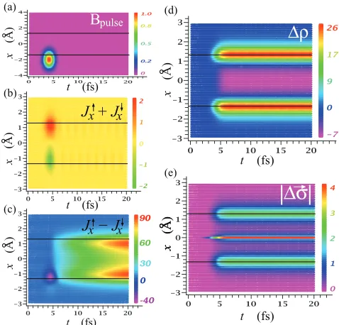
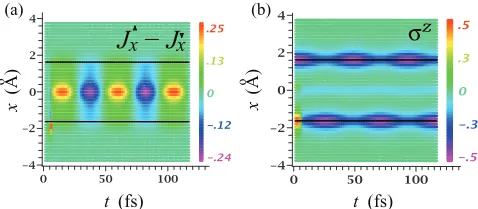
III. IMPLEMENTATION AND CALCULATIONS FOR H2 In this section we will consider a stretched H2molecule with a fixed bond length ofd =2.6 ˚A (protons are always frozen during simulation). The typical outcome of the described above TD-SDFT simulation scheme is presented in Fig. 2 in the form of two-dimensional contour plots representing the stacked-together snapshots of the one-dimensional distribution of a dynamical observable (its instantaneous expectation value) along the molecular axis as a function of the simulation time (in the horizontal direction). This can also be seen as a space-time visualization of a set of trajectories. For instance, it shows that the inhomogeneous magnetic field pulse, used to generate noncollinearity from the LS ground state, produces a localized spin and charge redistribution. A comparison between the pulse geometry in Fig.2(a)and the charge and spin currents in the panels below shows little direct spatial correlation (e.g., the pulse is centered at −2 ˚A while the excitation is centered at−1.3 ˚A where the proton sits), and this demonstrates further the freedom available in the choice of the actual magnetic field distribution.26 _{It also shows that}

the relatively small charge and spin redistribution in the dimer closely follows the temporal shape of the pulse. After the the pulse dies out, only a tiny amount of charge sloshing between the two sites at very high frequency remains, as evident from Fig.2(b). The figure represents the charge current as the sum of the up-spin and down-spin components (with respect to the quantization axis set by the initial spin polarization att=0)

x

(A)

o

t (fs)

t (fs)

t (fs)

t (fs)

x

(A)

o

x

(A)

o

x

(A)

o

t (fs)

x

(A)

o

B

x

(A)

o

(a)

(c)

(d)

(e) (b)

x x

J + J

J − J

-40

0 30 x

60 90

|Δσ|

Δρ

FIG. 2. (Color online) Contour plots of the time evolution (early time) of the distribution along the direction of the bond (x) of (a) the external magnetic pulse, in units of 3 kT; (b) the charge current density; (c) thezcomponent of the spin-current tensor [see Eq.(18)] in the same arbitrary unit scale; and the variations with respect to the ground state of (e) the charge density ρ(x,t)≡

ρ(x,t)−ρ(x,0), in units of 0.03e/A˚3; and (d) the magnitude of the spin density (Euclidean norm)|σ(x,t)| = |σ(x,t)| − |σ(x,0)|, in units of 0.3(¯h/2)/A˚3. Note that soon after the magnetic pulse dies out, the system becomes nearly stationary with respect to charge transfer between the two sites.

of the expectation value of spin-current tensor in the direction of the bond (xaxis). The later currents are defined by only two scalar componentsJx↑ ≡J↑↑x andJx↓≡J↓↓x of the Kohn-Sham

spin-current tensor,

Jμνl (r)=

n,m

ˆ

σμν n,m⊗jˆ

l n(r)

KS, (18)

where l and m∈ {x,y,z}, μ and ν∈ {↑,↓}, ˆjn(r)= ¯ h

2mi

[∇nδ(r−rn)−c.c.] is the orbital current operator for thenth

electron, ˆσn is its spin operator, and we have omitted the

implicit time dependence for simplicity. Note that while the charge current drops down close to zero after the pulse, the spin current builds up. After the pulse-coherent depletion of the longitudinal spin in the site more exposed to the pulse (the site at−1.3 ˚A), a unidirectional spin current is established. This corresponds to a transfer of spin-up along the positive x direction and of spin-down along the negativex direction. Hence, the the up-spin localized at the left site starts turning downward, while the down-spin on the right starts turning up. Figures2(d)and2(e)show that while this spin-rotation process is taking place, the distribution of the both the charge and the magnitude of the spin density after the pulse tend to remain stationary in space.

t (fs) t (fs) z

x

(A)

o

x

(A)

o

(b) (a)

J − J

100

0

50

100

60

σ

FIG. 3. (Color online) Contour plots as in Fig. 2but over the entire simulation time for (a) the zcomponent of the spin current density tensor (arbitrary units, as in Fig.1) and (b) thezcomponent of the spin density, in units of 300(¯h/2)/A˚3.

simulation box precesses about the total spin of the dimer with the same frequency). This is also evident from the sloshing of pure spin currents between the two atoms (see Fig. 3). The corresponding trajectories of the spin density integrated over atomically centered spheres are similar to those depicted in Fig. 1 (for a different pulse strengths) and are typically sinusoidal to a great level of accuracy within the duration of simulation (up to 200–250 fs).

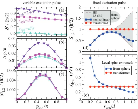
The properties of the linear transformationAwith respect to the mapping of the H2 spin-dimer dynamics onto classical degrees of freedom are demonstrated in Fig. 4. A set of noncollinear quasistationary dynamical states with anglesϕsph between the apparent local spins ranging from 0 to π are

0.6 0.7 0.8 0.9 1

S

/ (h

_ /2)

variable excitation pulse

0 0.01 0.02 0.03 0.04

Δ

ϕ

/π

0 0.2 0.4 0.6 0.8 1

ϕsph/π 1

1.002 1.004 1.006

|

σ1,2

| / (h

_ /2)

0 0.5 1 1.5 2

|

S1,2

| / (h

_ /2)

HS LS (BS) non-collinear transformed

fixed excitation pulse

0 0.2 0.4 0.6 0.8 1 1.2

r_sph/d

0 0.2 0.4 0.6 0.8 1

Jdyn

(eV)

from sphere transformed Local spins extracted:

rsph=d/2

r_sph=d/3

r_sph=2d/3 (a)

(b)

(c)

(d)

(e)

from sphere

FIG. 4. (Color online) Left-hand-side panels—Constants of mo-tion (i.e., showing only negligible numerical fluctuamo-tions after the pulse) as a function of the achieved apparent spin-misalignment angle

ϕsphfor three different radii of the sphere: (a) the magnitude of the

apparent local spin S; (b) the difference between the transformed and the apparent angles ϕ=ϕ−ϕsph; and (c) the transformed

local-spin magnitude|σ1,2|. Right-hand-side panels—As a function

of the sphere radius: (d) the apparent local-spin magnitude S in the two stationary collinear states and in the noncollinear state, and the transformed noncollinear spin magnitude (|σ1,2|) for the largest

sphere; and (e) corresponding Heisenberg constantsJdyn, as defined

by Eq.(10).

produced by applying pulses of different strengths from either the LS or the HS initial state. We find a systematic variation of the apparent local spin normS, which depends only on ϕsphalone, irrespective of the particular collinear initial state (whether LS or HS). The effect of the sphere radius on that dependence is significant [see Fig.4(a)]. In contrast, for the transformedspins the level of the normalization ofσi, achieved

by the transformation, is quite high regardless of the angleϕ (even when this is close toπ/2), and is practically the same for any size of integration sphere [Fig.4(c)]. The magnitude of thetransformedlocal spin varies by less than 1% for a range of rsph. Hence, it is practically constant on the background of the variation of the apparent spin magnitudeSat the two extreme HS and LS states as a function ofrsph[see Fig.4(d)]. At the same time the transformation of the angle shows a small but systematic dependence on the sphere radius [see Fig.4(b)]. The larger the spheres, the more of the overlap they capture and the greater the correction in the angleϕachieved by the transformation. The calculatedϕ between transformed local spins for any value ofrsphis always above the upper asymptotic limit of the apparent ϕ_sph as a function of decreasing r_sph. We find thatϕ_sph always tends to a saturation maximum for decreasingrsph. In fact, for the particular excitation depicted in the right-hand-side panels of Fig.4,ϕvaries just between 2.648 and 2.650 rad forrsphranging between 0.2d and 1.2d, while the change in the apparent angleϕ_sphis massive, i.e., it changes from 2.626 rad down to 0.789 rad (this data is not presented on the graph).

Figure 4(e) shows the resulting correction in the corre-sponding exchange parameterJdyn, defined as in Eq.(10). It demonstrates that the usage of theapparent local spins for evaluation ofJ_dynis rather arbitrary: the dependence on the sphere radius is very strong (for instance, in the large radius limitJdynunderstandably tends to 0). In contrast, by using the transformed quantities,Jdynas a function ofrsphis practically constant with a variance of less than 0.15% (for the case depicted in Fig.4,J_dyn=0.3413±0.0005 eV averaged for the 11 values ofr_sph in the range from 0.2d to 1.2d). Note that the linear transformation does not change the observed angular frequency of local spin precessionωfit. This is because any spatial portion of spin density in the noncollinear state precesses at the same rate.

ϕ/π

(A)

o

x

ϕ/π

( = 0)

x

ρ

(a)

Δρ

~ −cos

ϕ

Fit

FIG. 5. (Color online) Dependence on the dynamically generated angleϕof (a) the variation of the electron density distribution along the bond axisxwith respect to the low-spin state, whereρ(ϕ,x)=

ρ(ϕ,x)−ρ(0,x). Locations of the nuclei are marked by the black lines. (b) The electron density atx=0, compared to a cosine function (blue dashed curve) and fitted (least-squares) by a two-parameter function:Acosϕ+Bsin2_{ϕ(green curve). The units forρandρ}

are 0.3e/A˚3.

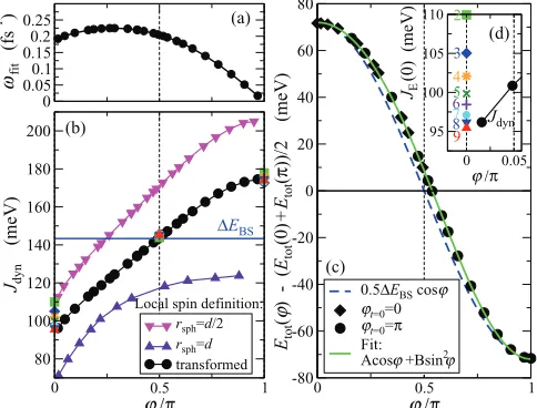
We now move to analyze the corresponding results for the exchange parameterJdyn, calculated from the dynamical simulations initiated with different magnetic pulses, giving rise to different anglesϕ. In Fig.6(a)we present the precession frequency ω_fit, while in Fig.6(b)isJ_dyn, as calculated from Eq.(10). Clearly bothωfitandJdyndepend sensitively on the angle between the two spin moments. The tendency towards zero forωfitforϕ →π is also present in the classical model [see Eq. (9)]. Unlike what is subsumed in the latter, the reversely calculated J_dyn is not constant with ϕ, indicating that our quantum system, simulated with TD-SDFT, deviates

0 0.05

ϕ /π

95 100 105 110

JE

(0) (meV)

0 0.5 1

ϕ /π

-80 -60 -40 -20 0 20 40 60 80

Etot

(

ϕ

) - (

Etot

(0)

+

Etot

(

π

))/2 (meV)

0.5ΔEBS cosϕ

ϕt=0=0

ϕt=0=π

Fit: Acosϕ+Bsin2_ϕ

0 0.05 0.1 0.15 0.2 0.25

ωfit

(fs

-1 )

0 0.5 1

ϕ /π

80 100 120 140 160 180 200

Jdyn

(meV)

rsph=d/2

rsph=d transformed Local spin definition:

(a)

(b)

(c) ΔEBS

(d)

J_dyn

2

3 4 5

6 7

8

9

FIG. 6. (Color online) Dependence on the dynamically generated angleϕof (a) the extracted frequency of rotationωfit. (This is the

same for theapparent as well as thetransformedspins.) (b) Jdyn

extracted from the spin trajectories [Eq. (10)]. (c) The total TD-SDFT energy (long-time value) with respect to the averageEtotvalue

between the LS and the HS states, i.e., Etot(ϕ)−(EHS+ELS)/2.

(d) Consecutive approximations toJdyn(ϕ=0) from Eq(19)using

the seriesn_i=0cicosi_{(ϕ) of increasing order up ton=9 as a fitting}

function for Etot(ϕ). Marked in panel (b) is also EBS=EHS− ELS=143.4 meV and the results for the exchange constant based

onEtot(ϕ) derivatives as in Eq.(19)(colored symbols atϕ=0 and ϕ=π).

from the classical one. Intriguingly, however, the dynamical exchange seems to agree perfectly with that calculated by Eq. (6) (the broken-symmetry approach) for ϕ=π/2, i.e., when the two local spins are orthogonal to each other. Note also that, once again, theapparentlocal spins cannot be used here, since the variations inJdynwith the choice of integration radius are very large.

A deviation from the classical Heisenberg model is found in the dependence of the total energyEtoton the angleϕbetween thetransformedlocal spins. Note that here we considerE_tot in the long-time limit, i.e., long after the external field pulse has extinguished. In this limitEtotis a constant of motion with numerical fluctuations after the first 100 fs, being typically smaller than 10−6 _{eV. The dependence of the total energy} Etot(ϕ) clearly deviates from the characteristic cosine form of the classical Heisenberg model [Fig.6(c)]. However, as we have found for the charge density [see Fig.5], also for Etot the best fit of the dynamical quantities is obtained by including higher-order harmonics, with already a remarkably good agreement at the level of the second harmonic (∝sin2_ϕ, note that with the use of sin2_{ϕ the offset of the fit is} 0). The deviation of the total energy from the Heisenberg model (∝cosϕ) can be attributed to a combination of factors. The Heisenberg model returns the energy of two localized electrons as the scalar product of their corresponding local spin operators.14_{Clearly, any definition of the local spins in terms of}

the expectation values of spin density and the correspondingϕ is an approximation. In addition, the total energy of the system in the noncollinear spin state is approximated here with the choice of the LSDA for the exchange-correlation potential.

A similar deviation from the Heisenberg model was found also by Peralta and Barone11 _{for several different spin-dimer}

complexes. They noticed that a systematic improvement of the agreement between the DFT results and the classical Heisen-berg model is achieved as the approximation for the exchange and correlation functional improves. In particular, a more Heisenberg-like behavior is found for hybrid functionals, such as B3LYP.27 _{This could be anticipated, since in hybrid}

func-tionals the spurious self-interaction, which is present in LSDA, is partially removed and the electron charge gets more local-ized at the nuclear sites.28 _{In brief, hybrid functionals return}

an electronic structure closer to that underpinning the classical Heisenberg model. In any case, a variation ofJ(evaluated from the second derivative of the total energy with respect toϕ) be-tween the values calculated around the LS state or those around the HS state was found for all functionals. This variation has the same sign as our corresponding quantity, calculated as

JE(ϕ)≡ 1 2S2

d2_E tot(ϕ)

dϕ2 cos(ϕ). (19)

From Fig.6(c)it appears that|JE(0)|>|JE(π)|, since the total energy as a function of ϕ lies above the Heisenberg cos-type dependence (the dashed curve), both approaching ϕ=0 and ϕ=π. We now demonstrate that this variation is consistent quantitatively with the exchange couplingsJdyn extracted from the dynamical trajectories via Eq. (10). In fact, if we use just the cosine part of the Fourier series

n

[see Fig.6(d), inset of Fig.6(c)]. This is a direct evidence that the spin dynamics of the molecule, excited and mapped out as described, indeed probes the spin-dependent energy surface of the system. In the vicinity of the HS and LS state, the agreement ofJ_dynand the Heisenberg model approximation of the total energy is remarkable. Furthermore, the fact thatJdyn closely matches the broken-symmetry result atϕ=π/2 can be understood by using the fitting cosine series to define the correspondingJE(π/2) throughdE(ϕ)/dϕatπ/2. Clearly, the latter is zero for the higher-order terms in the cosine series and hence J_E(π/2)=c₁. This is also by definition the broken-symmetry result for J. In conclusion, we find that the Heisenberg spin interaction is the governing mechanism for the ab initiospin dynamics of stretched H2. There are, however, obvious deviations over the whole span ofϕ from 0 toπ. In particular,E_tot(ϕ) contains higher-order contributions from the cosine-only Fourier series overϕ, besides the Heisenberg-type cosϕdependence.

A. Variation with distance

The hydrogen molecule has had a special role in quantum chemistry as a basis for understanding the chemical bond. It is well known that the Heitler-London theory of molecular bonding incorrectly produces a spin-triplet ground state in the dissociation limit,14_{because it omits the electron correlations.}

In the other limit, the Hartree-Fock molecular-orbital wave function fails due to an overestimation of the ionic contribu-tion. The ground state of the dissociating H2has a significant multiconfigurational character and it is still an unsolved problem for DFT.29_{Furthermore, the problem for the exchange}

coupling in H2 is the one for the spin-flip excitation energy 1+

g →3u+. The standard ALDA in TD-DFT is found to have

severe weaknesses and it badly underestimates the excitation energies in the dissociation limit.30,31 _{Limiting ourselves to}

the noncollinear ALDA, the aim of our work is not to offer an accurate alternative evaluation of the exchange coupling in H2, but to demonstrate a first attempt to relate the Heisenberg J to the actual spin trajectories calculated from TD-SDFT. It is well known that LSDA has serious shortcomings in describing long-distance exchange and correlation effects29

and our dynamical analysis cannot improve on these. For the sake of completeness in demonstrating our method’s applicability to H2, in Fig. 7 we present our results for the distance dependence of the exchange coupling in H2at medium distances (2–3 ˚A) and compare those to a number of previously published results, obtained at different levels of approximation. Our static broken-symmetry LDA result lies nearly in the middle between the leading term in the perturbative calculation ofJobtained with the surface integral method32and the exact variational result for the first spin-flip excitation energy.33

As discussed above, the value of our dynamical Heisenberg parameter J_dyn depends strongly on the angle ϕ. We show the entire span ofJdyn values between some of the smallest and some of the largest angles obtained (pulses are purposely chosen as to produce angles of nearly the same magnitude for alld). The variation inJdyn is significant on the background of the method-dependent variation, but it is systematic and the relative magnitude of the variation with respect to the mean value is nearly constant for all the bond lengths. Notably,

2.2 2.3 2.4 2.5 2.6 2.7 2.8 2.9 3 3.1 3.2

dH-H (Å)

0.1 1

Δ

EBS

,

Jdyn

(eV)

ΔEBS (LDA) J_dyn, 0.025π <ϕ< 0.03_π J_dyn, 0.97π <ϕ< 0.98π

E(3Σu+) - E(1Σg+) J (surface integral method) (a):

(b): (c): (d): (e):

FIG. 7. (Color online) Comparison of the distance dependence of the exchange coupling in H2calculated as (a) broken-symmetry

energy difference from Eq.(6)obtained by static LSDA calculations; (b and c)Jdynfrom Eq.(10)for anglesϕvery close to 0 and toπ,

respectively; (d)ab initiovariational calculation of ground state and first excited-state total energies by Kolos and Wolniewicz (Ref.33); and (e) the leading term in the surface integral method by Herring and Flicker (Ref.32).

the broken-symmetry LSDA value at any distance is always rather well reproduced by our dynamical calculation for angles ϕ≈π/2.

IV. RESULTS FOR THE H-He-H TRIMER

We now apply the dynamical scheme discussed so far to another system, namely, the hypothetical H-He-H molecule. This is the simplest possible model system presenting a higher-order spin-spin interaction, e.g., the two H electrons interact via the superexchange mechanism14_{across the closed-shell He}

atom. There are no experimental observations for H-He-H, but it is a good test case for new quantum chemistry methods,10 as full configuration interaction calculations exist34,35 _for

comparison. Here, as in many other works in the literature, we consider the most-widely-studied H-He distance of 1.625 ˚A.

In general, our results for H-He-H are similar to those for H2. Again, after the application of the spatially asymmetric magnetic field pulse, the spins of the hydrogen electrons become misaligned by an angleϕ and start to precess about the total spin at a steady angular frequency. Figure8shows the

x

(A)

o

t (fs) t (fs)

x

(A)

o

z

x x

(a) (b)

J − J

σ

FIG. 8. (Color online) Exactly analogous graphs to those in Fig.3but for H-He-H withdH−He=1.625 ˚A. Note that the exciting

magnetic pulse is strong enough to nearly reverse the spin of the H atom it is applied to. This results inϕ=0.33π and σz _{at both}

(A)

o

x

ϕ/π ϕ/π

( = 0)

x

ρ

Δρ

ϕ

(b)

Fit

~ cos

(a)

FIG. 9. (Color online) Exactly the same graphs and units as in Fig.5but for H-He-H withdH−He=1.625 ˚A.

long-time oscillations of the spin density and the oscillating z-polarized spin currents along the bond axis. The spin-current distribution is qualitatively different from that of H2in Fig.3, since it now peaks at the He atom instead of the sites bearing the localized spins. This provides a certain insight into the indirect exchange mechanism in H-He-H. Similarly to the case of H2, we extract the local spins at the hydrogen sites by using the linear transformation of Eq. (14). Also, in this case the transformation seems to work well since it produces consistent results and integration-volume-independent local spins (expectation values), anglesϕ, and correspondingJdyn. The variation of electron density along the bond axis as a function ofϕobtained in the long-time limit is shown in Fig.9. This reveals a density-level signature of the superexchange. As the spin state goes from LS to HS, the charge density at the He atom splits spatially and the two He electrons show a tendency to pair up with the uncoupled hydrogen electrons in the interstitial regions. The profile of the local charge density variation with ϕ at the center of symmetry (the He site) is again an approximate cosine [Fig.9(b)]. Note that the phase here is reversed with respect to that of Fig. 5(b). In fact, this exact profile, characteristic of the spin-pair formation, appears throughout the simulation box, albeit with different phase or amplitude. It appears that the deviation from a perfect cosine is much less pronounced here compared to the case of H2 (although we find again some higher-order harmonic contributions). Similarly, the profile of Etot(ϕ) fits to cosϕ better than that for H2. In fact, by using only one additional harmonic to the fitting function, namely,Acosϕ+Bcos2_ϕ, we find that the corresponding JE [see Eq. (19)] agrees extremely well with the extrapolated values ofJdynatϕ=0 andϕ =π(see Fig.10). The relative variation of bothJEand J_dyn, calculated either near the LS or the HS state, with respect to their average values, is also much smaller than that found in H2[see Fig.6(b)].

There can be two factors for the improved agreement to the Heisenberg law, namely, the increase of the H-H distance in this case (2.6 ˚A for H2 versus 3.25 ˚A for H-He-H), offering the possibility for a better localization of the spins, and the contribution of the superexchange spin-spin coupling.14 Concerning the first factor, clearly the presence of the He produces a different localization for the H-He-H trimer with respect to H2 for the samedH−H. A measure for

such localization is the integral of the spin density over a hydrogen-centered sphere of radius d_H−H/2. Hence, for the HS state of H2 at 2.6 ˚A we find 0.849¯h/2 and for H-He-H

0 0.5 1

ϕ /π

75 80 85 90 95

Jdyn

(meV)

transformed

0 0.5 1

ϕ /π

-40 -20 0 20 40

Etot

(

ϕ

) - (

Etot

(0)

+

Etot

(

π

))/2 (meV)

0.5ΔEBScosϕ Fit: Acosϕ+Bsin2ϕ

0 0.1 0.2

ωfit

(fs

-1 )

Local spin definition:

(a)

(b)

(c)

FIG. 10. (Color online) Same graphs as in Fig.6but for H-He-H withdH−He=1.625 ˚A. The broken-symmetry energy difference

marked in panel (b) isEBS=EHS−ELS=85.5 meV. The blue

squares correspond toJEfrom Eq.(19)with the fitting function in

panel (c), the blue broken line.

at 3.25 ˚A the apparent spin is 0.931¯h/2, which suggests the latter should indeed be more Heisenberg-like. However, at small distances, H-He-H shows much larger deviations from the Heisenberg model compared to H2 for the same dH−H. (See, for instance, Fig.13in the Appendix, where the case of H-He-H withdH−H=2.6 ˚A is discussed.)

As a quantitative measure of the deviation from the Heisenberg model, we take the variation ofJ_dynbetween the HS and the LS spin on Fig.10(c). This has the same sign and is comparable in magnitude to the constrained-spin DFT result of Peralta and Barone.11_{It is further suggested in Ref.11that}

a significant portion of theJ variation is related to the LSDA approximation, becauseJ_E(π)−J_E(0) can be reduced from about 6% of the averageJ value to less than 1% with the use of a hybrid exchange correlation functional such as B3LYP.

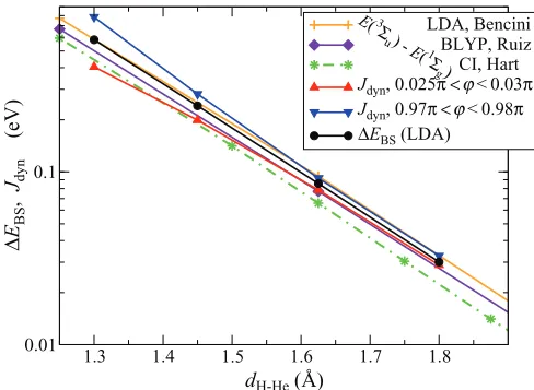
We finally present results for the dependence ofJdyn on the He-H distance,dH−He. In Fig.11the calculatedJdynin the vicinity of the two collinear spin states are compared to

broken-1.3 1.4 1.5 1.6 1.7 1.8

dH-He (Å)

0.01 0.1

Δ

EBS

,

Jdyn

(eV)

LDA, Bencini BLYP, Ruiz CI, Hart J_dyn, 0.025π <ϕ< 0.03π J_dyn, 0.97π <ϕ< 0.98π

ΔE_BS (LDA) E₍3

Σ_{u) -}

E₍1

Σ_g)

symmetry DFT10,34 _{and the exact configuration interaction}

results available in literature.35_{Similarly to Fig.7, the average}

Jdyn(or approximately its value forϕ=π/2) agrees well with the LSDA broken-symmetry result. Here we find that at very large distances the relative variation ofJdynwithϕdecreases and it converges towards our LSDA broken-symmetry value as d_H−H increases. Such convergence is not found for the case of H2 for the range of separations presented in Fig. 7. Hence, at very large distances our dynamical measure of the spin-spin interactionJdynsuggests that the superexchange part of the spin-spin interaction in H-He-H becomes increasingly more Heisenberg-like as bond length increases. In fact, we find that for the same dH−H, while the relative variation [Jdyn(π)−Jdyn(0)]/Jdyn(π/2) for H-He-H is about 20% larger at d_H−H=2.6 ˚A than that for H2, it becomes nearly 3 times smaller than the latter atdH−H=3.2 ˚A. At the same time, the absolute deviationJdyn(π)−Jdyn(0) for H-He-H is always significantly larger than that for H2for the samedH−H.

V. CONCLUSIONS

We have demonstrated that the spin dynamics of two simple spin dimers, as calculated on the basis of TD-SDFT within the adiabatic LSDA, is rather simple and understandable through a classical model. A noncollinear spin state can be created with inhomogeneous magnetic field pulses and this retains the noncollinearity in the long-time limit. The long-time spin dynamics is thus a harmonic precession in which the noncollinear spin density rigidly revolves about the total spin of the dimer and all the relative angles remain constant in time. Hence, the trajectories of the localized atomiclike spins, independently from their particular definition, map well onto the classical Heisenberg model. In order for this mapping to be used for the extraction of Heisenberg exchange parameters, the actual definition of local spins is important.

We have showed how a linear transformation, based on the HS and the LS collinear states and the direct integration of spin density over atomically centered spheres, can be used to extract the directions of two localized spins. When defined in this way the latter are, to a good degree, independent of the integration sphere used for their definition. This also remains valid for the corresponding dynamically defined exchange parameter J_dyn, even for a range of distances where the overlap of the atomic wave function is significant. Such defined exchange parameters agree well with the results from constrained DFT around the LS and the HS states and with broken symmetry based on the total LSDA energy. We do acknowledge that the actual form of the exchange parameter depends on the choice of exchange and correlation functional used and that our dynamical method does not remedy the shortfall of local and semilocal functionals. We believe that the dynamical method highlighted in this paper, together with generating a quantitatively relevant estimate of J, could potentially provide a straightforward verification for the applicability of the Heisenberg spin model to a range of spin-polarized nanoscaled systems accessible to TD-SDFT calculations (a few hundreds of atoms). Furthermore, it offers a possible strategy for mappingab initiosimulations on the widely used atomistic Landau-Lifshitz-Gilbert micromagnetic models for spin dynamics.

ACKNOWLEDGMENTS

This work has been sponsored by the the European Union under the Cronos project (No. 280879). The authors wish to acknowledge the SFI/HEA-funded Irish Centre for High-End Computing (ICHEC) for the provision of computational facilities and support.

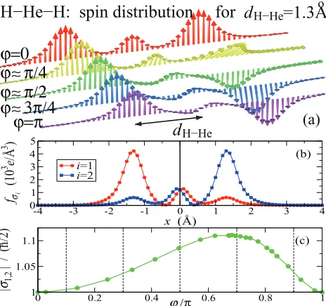
APPENDIX: DEPENDENCE OF THE CALCULATED J’s ON THE LOCAL SPIN DEFINITION: THE H-He-H CASE We elaborate here on the procedure for extracting the local spins and the exchange parameters for the H-He-H molecule. The leading exchange mechanism in this system is not the direct one but the superexchange, which depends on the kinetic energy matrix element between the atomic orbital at the two magnetic sites. It is then not cleara prioriwhether the linear transformation used to eliminate the dependence on the wave-function overlap in H2 is transferable to this case. Indeed, for H-He-H the spin-density snapshots in the long-time limit show a complex texture with multiple peaks and valleys around the He site and the interstitial regions (see Fig.9). The main approximation, subsumed in the linear transformation, that the HS and LS state have approximately the same single-electron density distributions (but not spin direction), seems likely to be violated if one looks at the transformation of the spin distribution between the HS and the LS state as illustrated in Fig.12(a). This, however, is not the case, and we find that the average variation between the actual density distributions of the LS and HS collinear states at any point in the simulation box is below 5% ford_H−He=1.3 ˚A. With this result at hand, we verify numerically that the linear transformation, described in Sec.II D, is still an adequate choice for the local spin definition even at relatively small interatomic distances.

Our first criterion for assessing the adequacy of the local spin definition is the fact that the absolute values of the spins and the angles, obtained through the linear transformation, do not depend on the choice of the sampling spatial volume, e.g., on the radius rsph of the sphere used to integrate the spin density. We find numerical evidences that this criterion is fulfilled even for small H-He distances where the overlaps are significant. In the top panels of Fig.13we compare the total energy profiles as a function of the angleϕ between the two hydrogen local spins, forϕdetermined directly from the ap-parent spins in an extremely small sphere (rsph=0.05dH−He),

in an extremely large sphere (rsph=dH−He), and the case of

ϕdetermined after the linear transformation (the blue squares in the graphs). For instance, in the more problematic case of small separationdH−He=1.3 ˚A, the average relative variation in the calculatedϕ (after the linear transformation) is below 0.5% for a variation ofrsph between 0.05dH−He anddH−He.

ϕ π/4

ϕ π/2

ϕ 3π/4

-4 -3 -2 -1 0 1 2 3 4

x (Å)

0 1 2 3 4 5

fσi

(10

3 e/Å 3 )

i=1 i=2

0 0.2 0.4 _ϕ/π 0.6 0.8 1

1 1.05 1.1

|σ1,2

| / (h

_ /2)

(b)

(c)

∼∼

∼∼

∼∼

d

d

ϕ=0

ϕ=π

(a)

=1.3A

H−He−H: spin distribution for

FIG. 12. (Color online) (a) Snapshots of the long-time spin density along the axis of H-He-H for dH−He=1.3 ˚A. (Note that

individual illustrations are rigidly rotated about the molecular axis so that the leftmost spins in all snapshots are parallel to each other.) (b) The carrier functions of the two spin-density distributions s1(r) and s2(r) [see Eq. (12)], based on the HS and the LS

collinear states. (c) Variation of the magnitude of the local spin, defined as |σi| ≡ |Ci|

fσ_i(x)dx (which is identical for i=1,2 because of the symmetry), as a function of the angleϕ when the linear combinationC1fσ1(x)+C2fσ2(x) instead is used to fit the noncollinear distributions in panel (a). This result matches exactly |σ1,2|obtained through the linear transformation of Eq.(14).

much more classically. In the case of a large bond length all the E_tot(ϕ) curves (for different local sphere definitions) collapse onto one, which tends towards the ideal Heisenberg cosine law [see Fig.13(b)].

A second relevant criterion could be how well the definition preserves the magnitude of the local spin in the various noncollinear states. Ideally, if the spin-density distributions si(r) [Fig.12(b)], determined from the sum and the difference

of spin density between the LS and HS collinear states, are preserved in the noncollinear state (they only rotate), the linear transformation in Eq.(14)will not affect the spin magnitudes in the noncollinear states (σi are normalized by definition). The

result of the linear transformation ford =1.3 ˚A is presented in Fig. 12(c). Clearly, the variations from the norm of 1 are relatively small, with a peak at aboutϕ =2/3π, where the local spin is about 11% larger than its value atϕ=0 orϕ =π. As a final criterion, we consider how well the exchange couplingJ_E extracted from the total energy [Eq.(19)] agrees with the dynamical exchangeJ_dyn defined in Eq.(10). This comparison is presented in the bottom panels of Fig. 13. Here we also take into account the fact that different local spin definitions result in different values of the angleϕ. The magnitude of the local spins in Eq. (10)are assumed to be alwaysS =1/2. When analyzing such a direct comparison, we need to keep in mind that the values ofJEare associated

-101.2 -101 -100.8 -100.6

Etot

(eV)

-101.72 -101.7 -101.68 -101.66 -101.64

∝ cos(ϕ)

0 0.2 0.4 0.6 0.8 1

ϕ/π

400 600 800 1000 1200

J

(meV)

rsph=d

rsph=0.05d

transformed

0 0.2 0.4 0.6 0.8 1

ϕ/π

75 80 85 90 95

transformed

rsph=0.05d rsph=d

d_H-He=1.625Å

d_H-He=1.3Å

for model local spins: Jdyn

JE

Model for local spins:

shaded area curves: symbols + guiding lines:

(a) (b)

(d) (c)

(legend as above)

FIG. 13. (Color online) Comparison to an ideal Heisenberg cosine law (solid black curve) of Etot(ϕ) (total TD-SDFT energy

in the long-time limit) profiles with angles {ϕ} corresponding to different definitions of the local spins for two different bond lengths: (a)d=1.3 ˚A and (b)d=1.625 ˚A. CorrespondingJEvalues at the

two collinear spin limits [see Eq.(19)], for three different definitions of the local spins, are compared to the dynamical results forJdyn

(the area shaded in gray). The straight lines are just guides to the eye between the two values. The type of line is matched to the corresponding dynamical result (in or at the border of the gray-shaded region) for the same definition ofϕ.

with substantial inaccuracy, as they rely on a numerical second derivative. The error bars represent the standard deviation of a set of results (of about 20 entries) obtained by using either different forms of local interpolation (polynomial) around the end points (0 andπ) or global fits ofE_tot(ϕ) to Fourier cosine series of up to ninth order.

*_{[email protected]}

1_{I. Tudosa, C. Stamm, A. B. Kashuba, F. King, H. C. Siegmann,}

J. St¨ohr, G. Ju, B. Lu, and D. Weller,Nature (London)428, 831 (2004).

2_{A. Aharoni,Introduction to the Theory of Ferromagnetism(Oxford}

University Press, Oxford, 2001).

3_{J. Miltat, G. Albuquerque, and A. Thiaville in Spin Dynamics} in Confined Magnetic Systems I, edited by B. Hillebrands and K. Ounadjela (Springer, Berlin, 2003).

4_{S. V. Halilov, A. Y. Perlov, P. M. Oppeneer, and H. Eschrig,}

Europhys. Lett. 39, 91 (1997); S. V. Halilov, H. Eschrig, A. Y. Perlov, and P. M. Oppeneer,Phys. Rev. B58, 293 (1998).

5_{N. Kazantseva, D. Hinzke, U. Nowak, R. W. Chantrell, U. Atxitia,}

and O. Chubykalo-Fesenko,Phys. Rev. B77, 184428 (2008).

6_{U. Atxitia, O. Chubykalo-Fesenko, R. W. Chantrell, U. Nowak, and}

A. Rebei,Phys. Rev. Lett.102, 057203 (2009).

7_{B. Skubic, J. Hellsvik, L. Nordstr¨om, and O. Eriksson,J. Phys.:}

Condens. Matter20, 315203 (2008).

8_{D. Hinzke and U. Nowak,Phys. Rev. B61, 6734 (2000).} 9_{L. Noodleman,J. Chem. Phys.74, 5737 (1981).}

10_{E. Ruiz, J. Cano, S. Alvarez, and P. Alemany,J. Comp. Chem.20,}

1391 (1999).

11_{J. E. Peralta and V. Barone, J. Chem. Phys. 129, 194107}

(2008).

12_{E. Beaurepaire, J.-C. Merle, A. Daunois, and J.-Y. Bigot,Phys. Rev.}

Lett.76, 4250 (1996).

13_{A. Kirilyuk, A. V. Kimel, and T. Rasing,Rev. Mod. Phys.82, 2731}

(2010).

14_{K. Yosida, Theory of Magnetism (Springer-Verlag, Heidelberg,}

1996).

15_{E. K. U. Gross and W. Kohn, Adv. Quantum Chem. 21, 255}

(1990).

16_{L. M. Sandratskii,Adv. Phys.47, 91 (1998).}

17_{Z. Qian and G. Vignale,Phys. Rev. Lett.88, 056404 (2002).}

18_{A. Castro, H. Appel, M. Oliveira, C. A. Rozzi, X. Andrade,}

F. Lorenzen, M. A. L. Marques, E. K. U. Gross, and A. Rubio, Phys. Status Solidi B243, 2465 (2006).

19_{A. E. Clark and E. R. Davidson,J. Chem. Phys.115, 7382 (2001).} 20_{E. Ramos-Cordoba, E. Matito, I. Mayer, and P. Salvador,J. Chem.}

Theory Comput.8, 1270 (2012).

21_{M. A. L. Marques and E. K. U. Gross, in A Primer in Density} Functional Theory, edited by C. Fiolhais, F. Noqueira, and M. Marques, Lecture Notes in Physics (Springer, Berlin, 2003), Vol. 620.

22_{J. P. Perdew and A. Zunger,Phys. Rev. B23, 5048 (1981).} 23_{A. Castro, M. A. L. Marques, and A. Rubio,J. Chem. Phys.121,}

3425 (2004).

24_{K. Capelle, G. Vignale, and B. L. Gy¨orffy,Phys. Rev. Lett.87,}

206403 (2001).

25_{Note that this is valid for any component of the spin density, if there}

is no static homogeneous magnetic field applied. If there is, say, a homogeneous fieldBh=(0,0,Bh), the result remains valid only for

the spin-density component along the field, i.e., thezaxis, in this case.

26_{We find that as long as the magnetic field is not symmetric with}

respect to the center of the dimer, this qualitative result persists.

27_{A. D. Becke,J. Chem. Phys.98, 5648 (1993).}

28_{A. Akande and S. Sanvito,J. Chem. Phys.127, 034112 (2007).} 29_{E. J. Baerends,Phys. Rev. Lett.87, 133004 (2001).}

30_{O. V. Gritsenko, S. J. A. van Gisbergen, A. G¨orling, and E. J.}

Baerends,J. Chem. Phys.113, 8478 (2000).

31_{F. Wang and T. Ziegler,J. Chem. Phys.121, 12191 (2004).} 32_{C. Herring and M. Flicker,Phys. Rev.134, A362 (1964).} 33_{W. Kolos and L. Wolniewicz,J. Chem. Phys.43, 2429 (1965).} 34_{A. Bencini, F. Totti, C. A. Daul, K. Doclo, P. Fantucci, and}

V. Barone,Inorg. Chem.36, 5022 (1997).

35_{J. R. Hart, A. K. Rapp´e, S. M. Gorun, and T. H. Upton,J. Chem.}