Abstract
This paper illustrates the impact of ignoring survey design and hierarchical structure of survey data when fitting regression models. Data on child nutritional status from Ghana, Malawi, Tanzania, Zambia, and Zimbabwe are analysed using four techniques: ordinary least squares; weighted regression using standard statistical software; regression using specialist software that accounts for the survey design; and multilevel modelling. The impact of ignoring survey design on logistic and linear regression models is examined. The results show bias in estimates averaging between five and 17 per cent in linear models and between five and 22 per cent in logistic regression models. The standard errors are also under-estimated by up to 49 per cent in some countries. Socio-economic variables and service utilisation variables are poorly estimated when the survey design is ignored.
SSRC Applications and Policy Working Paper A03/07
Impact of estimation techniques on regression analysis: an application to
survey data on child nutritional status in five African countries
Impact of estimation techniques on regression analysis: an application to
survey data on child nutritional status in five African countries
Nyovani Madise1, Rob Stephenson2, David Holmes1, and Zoë Matthews1
1Department of Social Statistics, University of Southampton, Highfield, Southampton, UK, SO17 1BJ
2
Bill and Melinda Gates Institute for Population and Reproductive Health, Johns Hopkins Bloomberg School of Public Health, Baltimore, USA
Introduction
Many studies that analyse data from large surveys often use software designed for simple random samples. Such analyses fail to take into account the impact of the complex sampling design on
regression parameter estimates such that the conclusions drawn from these analyses can be
misleading. Many of the samples collected under the Demographic and Health Surveys (DHS)
programme are drawn using stratified multistage sampling designs , often with over-sampling of
smaller domains such as urban areas or some regions of the country (Institute for Resource
Development 1987). If the unequal probabilities of selection are ignored, inferences based on the
unweighted sample data may be biased since individuals from the over-sampled domains will have greater weight than is the case in the population.
The importance of accounting for the sample design in regression modelling has been widely
acknowledged in statistical literature (DuMouchel and Duncan 1983; Korn and Graubard 1995; Pfeffermann and La Vange 1989; Smith 1988; Skinner et al 1989). There are three elements of the
survey design that may have an effect on the regression estimates based on survey data: the sample
weights, stratification, and clustering (Korn and Graubard 1995). The sample weight associated
set can therefore be thought of as, approximately, the number of individuals in the population that
are represented by the sampled individual. Thus the sample weights act to correct sample data for
the unequal selection probabilities and failure to include these in the modelling process can lead to
estimates that are seriously biased for their corresponding population quantities.
Stratification can produce gains in precision. That is, a stratified design can lead to smaller
standard errors than a simple random sampling design if the observations within strata are similar.
If the stratification is ignored in the analysis the standard errors will be too large, hence the confidence intervals will be too wide, giving coverage greater than the nominal coverage. Cluster
sampling is often used in national social and demographic surveys, where the clusters are groups of
households derived from census enumeration areas or from well-defined communities. Clustering
is of both statistical and substantive importance. Individuals who belong to a particular cluster may be more alike than those of different clusters, such that the assumption of independence assumed in
ordinary regression techniques is violated. The failure to recognise the clustering of survey data
may lead to standard errors that are smaller than the true standard errors, and hence confidence
intervals may be too narrow, leading to erroneous model results.
The correlation of outcomes that may arise as a result of clustered data can also be of interest in
identifying potential determinants or causes of the outcome under observation. For example, the correlation of mortality risks within a family may indicate genetic frailty among its members. In a
data set, there may be many levels at whic h potential correlation may be expected. For example,
children may be nested in households, which are clustered in communities, so that correlation may
exist at both levels. The development of software to handle multilevel data has enabled researchers to quantify the correlation of outcomes of interest at various levels of social organisation.
There are several views in the literature on the ways to analyse complex survey data. Some argue
the strata in the design phase (Skinner et al 1989; Korn and Graubard 1995). In this approach,
models are used to mitigate the impact of the complex survey design and regression diagnostics are
used to assess the performance of the models. Other statisticians argue for a design-based
approach, where the complex design is controlled for explicitly through the use of weighted regression and appropriate software that can handle complex survey designs (Eltinge et al 1997).
Both approaches have merits and drawbacks. It has been suggested that the model-based approach
performs better than the design-based approach when the sample design is inefficient, for example,
when very few primary sampling units are selected per strata (Graubard and Casady 1997). Another situation when the model-based approach may be preferred is when the sampling weights
vary considerably, or when non-response is a significant problem. This approach requires
verification of the model assumptions through diagnostics, and is thus less often used by analysts of
large surveys (Eltinge et al. 1997).
The recognition of the complex survey design and the hierarchical structure of the data both make
an important difference to the modelling process and it is desirable that a model should be fitted
which incorporates both types of effect. Statistical packages for multilevel models such as MLwiN
(Institute of Education 2000), while capable of handling many levels of clustering, do not handle
weighted data well particularly where the sample weights are not independent of the cluster effect.
Pfeffermann et al. (1998) proposed methods of weighting in multilevel models but the appropriate software for these methods is still not available.
In this paper, data from DHS programmes conducted in Ghana, Malawi, Tanzania, Zambia, and
Zimbabwe between 1992 and 1994 are used to assess the determinants of child nutritional status. Three types of software are used: SPSS version 10 (SPSS Inc. 2000), the standard statistical
software commonly used in the social sciences; STATA release 7 (StataCorp 2000), statistical
software which includes specialist commands for analysing data from complex surveys; and
contrasts four estimation procedures and will argue a case for the eventual inclusion of the survey
design and the hierarchical structure of the data in the same modelling process.
Nutritional status of children
A series of demographic and health surveys conducted since 1984 have collected weight and height
data for children under five years as well as a wealth of other individual level information about
each child, their family and their household. Data from the DHS programme are particularly
suitable for comparative studies since they contain a similar core set of information although variations do sometimes occur as countries can choose to omit or add some questions. Of
particular importance to this study are the anthropometric measurements of children and their
mothers, socioeconomic characteristics of the households, breastfeeding patterns, and morbidity of
children.
To measure the nutrit ional status of the child anthropometric measurements are compared to
standard National Health Centre, Centre for Disease Control and World Health Organisation (NCDS/CDC/WHO) reference populations to obtain height-for-age z-scores. For example, a child
is regarded as being stunted if his or her height-for-age z-score is less than two standard deviations
from the median of the NCHS/CDC/WHO international reference population for the relevant sex
and age group. Stunting is an indication of long periods of inadequate dietary intake, often combined with repeated infection. To measure underweight and wasting, weight-for-age and
weight-for-height z-scores can be used as indicators.
In this paper, height-for-age z-scores and a binary variable for stunting (1=stunted) are used in the linear regression and logistic regression models, respectively. These nutritional status indicators
were chosen for illustrative purposes only but other indicators of nutritional status have been used
in the literature (McMurray 1996; Madise et al 1999). The percentage of children aged 1-35
months who were stunted, as defined by the above measure, in the five countries are: 22 in
[FIGURE 1 ABOUT HERE]
Description of the survey designs
Most DHS surveys use stratified multistage cluster sampling. At the first stage, the country is
stratified into subgroups (or strata) that are as similar as possible and in many countries,
stratification is based on geographical areas (such as regions or provinces and urban or rural
residence). Each stratum is divided into units, which in many cases are census enumeration areas. From these standardised segments of roughly the same size are created (Macro International,
1996). From each stratum, units known as ‘primary sampling units’ (PSUs) are chosen with
probability proportional to size, where the size is the number of standardised segments or
households. One segment is randomly selected from each PSU. The number of PSUs selected from each stratum is based on proportional allocation, with the same sampling fraction in each stratum to
create a self-weighting sample. In some cases varying sampling fractions are used so that some
strata are over-sampled or under-sampled. At the second stage, all households in a segment are
listed and a fixed number are selected using systematic sampling. All women aged 15-49 years in
the selected households are eligible to be included in the interviews.
The Ghana survey used the same sampling fraction in each stratum so that the resulting sample is self-weighting (Ghana Statistical Service and Macro International 1994). In the four remaining
surveys, some strata were over-sampled (unequal sampling fractions) so that the samples are not
self-weighting. These samples require weighting when making national-level estimates. The
response rates for the surveys under consideration averaged approximately 95 percent. Full details of the precise numbers of households and women that were selected are reported in the respective
DHS country reports.
Methods
Height-for-age z-scores for children aged 1-35 months (continuous outcome) are regressed using
the same set of socioeconomic and demographic variables in each country (see Table 1 for a full
list of the variables used). The choice of the explanatory variables was determined by earlier work
on the determinants of nutritional status among African children (Madise et al 1999).
[TABLE 1 ABOUT HERE]
Ordinary least squares (OLS) regression (which we label Model AI) is applied using the SPSS statistical package. This method treats the data as if they had been sampled using simple random
sampling. The variables used during stratification are included as explanatory variables as
suggested by Skinner et al (1989). The second analysis (Model AII) is a weighted least squares
regression, performed using SPSS. This approach produces unbiased parameter estimates but the standard errors are incorrect. In the third approach (Model AIII) we use STATA to account for the
unequal sampling probabilities, stratification, and the clustering of individuals within primary
sampling units. This approach produces unbiased estimates and appropriate standard errors for the
design. The fourth analysis uses MLwiN to fit a three-level model (Model AIV) to account for the
hierarchy in the data. The three levels are the primary sampling unit (hereafter called
“community”), the family or household, and the child.
Corresponding analyses are performed using a binary dependent variable (stunted or not stunted).
Model BI is the standard logistic regression from SPSS, Model BII is the weighted logistic
regression, Model BIII is the logistic regression that accounts for the survey design, and Model
BIV is the three-level logistic regression model using MLwiN.
Although simple random samples are the simplest to analyse, they are often very expensive and are
rarely used for large surveys. Complex designs are often cheaper in comparison but there is a cost
loss of efficiency is the ratio of the standard error of an estimate under the comple x design to the
standard error of the estimate assuming that the sample was drawn by simple random sampling.
This is known as the design factor or design effect (deft), and is estimated using the formula:
srs c
vˆ
vˆ
=
deft
where
vˆ
c is the estimated variance of the parameter estimate under the complex survey design(Models AIII and BIII) , and
vˆ
srs is the corresponding estimated variance under simple randomsampling (Models AI and BI). For example a design factor of two would suggest that the standard
error under the complex design is twice that which would have been obtained if simple random sampling had been used. A design factor of less than one would indicate that the complex survey
design was more efficient than simple random sampling for estimating the quantity in question.
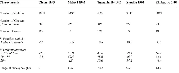
Finally, the data are clustered (that is children within families, and families within communities) so that it is important to account for this hierarchy (see Table 2). On average, about nine per cent of
the households have two or more children in the sample. Similarly, about 40 per cent of the
clusters of households have ten or more children, except in Ghana where the percentage is only
about seven. The degree of clustering of nutritional status of children within a family can be measured from the multilevel models using the intra-family correlation coefficient. This is the
ratio of the family-level variance to the total variance. Similarly, the intra-community correlation
coefficient (the ratio of the community-level variance to total variance) measures the homogeneity of nutritional status within communities. For the logistic regression models, the child level
variance is assumed to equal
3
2
π
as proposed by Im and Gianola (1988).
[TABLE 2 ABOUT HERE]
As preliminary analyses, 95 percent confidence intervals for the mean height-for-age z-scores were
calculated using two approaches: confidence intervals calculated using STATA, which account for
aspects of the survey design, and those calculated assuming that the data come from simple random
samples (see Figure 2). It can be seen that generally, the confidence intervals that do not account for the survey design are narrower than those that account for the survey design. In particular, the
confidence intervals for Malawi do not overlap, indicating that if the design of the survey is
ignored, differences may appear more significant than they really are.
FIGURE 2 ABOUT HERE
Parameter estimates for linear models
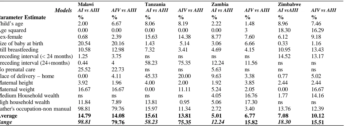
When the weights are ignored, the parameter estimates may be biased. The degree of the bias can therefore be measured by the difference in the estimates between the model that accounts for the
weights and the models that ignore the weights. In this section, we compare for each country, the
parameter estimates for Model AI against Model AIII to estimate the degree of bias as a
consequence of ignoring the weights. A comparison is also made between estimates from the
three-level linear model (Model AIV) and Model AIII. Model AII, the weighted regression,
produces unbiased estimates that are identical to those from Model AIII. From Table 3, it can be
seen that the degree of bias in the estimates as a consequence of ignoring the sampling weights varies. On average, the bias is highest in Tanzania and Malawi and lowest in Zambia.
[TABLE 3 ABOUT HERE]
For the case of Malawi, treating the data as if they were obtained from a simple random sample
(Model AI) result in an overestimation by nearly 100% of the estimate for the father’s occupation
(non-manual versus manual). This estimate is significant at a five per cent level in Model AI but
mother received prenatal care. The estimate for this variable in Model AI is about 25 per cent
higher than that from Model AIII. In contrast, the estimate for the size of the baby at birth is
underestimated in the models that do not account for the sampling weights.
In the linear models, the estimate for the sex of the child for the Tanzania data is underestimated
when the weights are not accounted for. The estimate for the parameter for preceding birth
intervals of 24 months or longer is significant at a five per cent level in Models AI and AIV but not
significant, even at 10 per cent level in Model AIII. The magnitude of the bias is also quite large. The estimates for the place of delivery are larger in magnitude (and therefore more significant)
when the sampling weights are ignored.
The difference of the estimates across the models for Zambia and Zimbabwe are generally smaller
than those found in the Malawi and Tanzania data. Since the Ghana sample was self-weighting, there were no differences in the estimates across the four models and although the standard errors
varied, the significance of the models did not change across the four approaches.
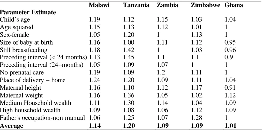
Standard errors for linear models
In this section, comparisons of the standard errors are made between the four models. The ratios of
the standard errors under the complex survey design (Model AIII) to the standard errors from
ordinary least squares (Model AI) are presented as design factors in Table 5. These design factors, are consistently greater than one, except for Ghana, showing that ignoring the survey design leads
to underestimation of the standard errors. On average, the design factors are largest in the Tanzania
data, followed by Malawi, and are smallest in Ghana.
[TABLE 4 ABOUT HERE]
When the weighted least squares regression is performed (Model AII) the standard errors produced
AIII. On average, the standard errors from Models AII and those from Models AIV were smaller
than those from Model AIII by about 13 per cent (results not shown). This suggests that if only
some components of the survey design (e.g. weights or clustering only) are accounted for in the
analysis, the standard errors may still be underestimated. This will result in more significant results than is the case.
Parameter estimates for logistic models
On average, the bias is larger for logistic regression than for the linear models. Again the
magnitude of the bias is largest for Tanzania, followed by Malawi and is least in Zambia (see Table
4). The estimates for the length of the preceding birth interval, the place of delivery, household
wealth and the father’s occupation show greater bias than the rest of the variables.
[TABLE 5 ABOUT HERE]
As with the linear models, some of the parameter estimates are biased when the weights are
ignored to the extent that the significance of the parameter is changed. For example, for the
Malawi models, the estimate for short preceding birth intervals (< 24 months) is significant at the
five per cent level in Model BI but insignificant in Model BIII. Conversely, the estimate for ‘medium household wealth’ is significant in Model BIII but not Model BI and the degree of the
bias is nearly 40 per cent. Again the estimate for father’s occupation in the Malawi models shows
a high degree of bias when the weights are ignored.
The sex of the child in the Tanzania data is estimated with bias by about 24 percent in the ordinary
logistic regression model (Model BI) and by about 20 percent in the three-level logistic regression
model. The estimate for preceding birth intervals of 24 months or longer varies greatly between
delivery, the estimate is overestimated by nearly 100 per cent in Model BI and was highly
significant (p < 0.001) but not significant in Model BIII. There are also large differences in the
estimates for the father’s occupation across the models for Tanzania.
For the Zambian models, the largest biases are for estimates of whether or not the mother received
prenatal care and the place of delivery. The differences in the parameter estimates across the
models for the Zimbabwe data are relatively small except for age-squared and maternal weight but
these are based on small values. All the four models for the Ghana data produced similar results.
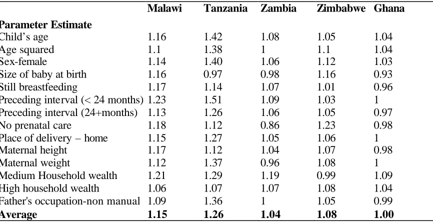
Standard errors for logistic models
The design factors for the logistic regression models (Model BIII versus Model BI) are presented in Table 6. Across the countries, the general pattern is similar to the linear models. Again, the
standard errors from Model BIII are larger than those from Model BI and this is reflected by design
factors exceeding one. Some of the design factors are less than one, indicating that the complex
survey design is produces more efficient estimates. A comparison was also made between the
standard errors of Models BII and BIII and also between BIV and BIII. The results (not shown)
indicate that the standard errors from the weighted logistic regression and the three-level logistic
regression models are slightly smaller (by about five per cent, on average) than those from the models accounting for the survey design.
[TABLE 6 ABOUT HERE]
Family and community level clustering of nutritional status
The three-level models (Models AIV and BIV) allow for the estimation of the correlation of
nutritional status between children of the same family and also between children of the same
Malawi, 0.28 Tanzania for, 0.30 for Zimbabwe and 0.33 for Zambia. Only in Ghana was this
intra-family correlation not significant. At the community level, the correlation was smaller, averaging
about three per cent. From the logistic regression models, the intra-family effects were much
weaker, ranging between four per cent in Tanzania to about 14 per cent in Zimbabwe. The intra-community correlation coefficients averaged about two per cent.
Discussion
Many researchers have demonstrated the pitfalls of ignoring the survey design when analysing data (Chambers 1986; Skinner et al 1988; Brogan 1998; Eltinge et al 1997) but few have performed
multi-country comparisons (Lê and Verma 1997). The impact of complex designs on regression
modelling is now a subject of interest among social scientists since statistical software for properly
handling complex survey designs is available. Many social and demographic surveys use stratified multistage sampling and commonly use the regions and/or the place of residence to stratify the
population. Such designs tend to be informative for many health outcome variables such as
nutritional status, mortality, and fertility so that inferences based on analyses that ignore the design
of the survey can be misleading.
These results have demonstrated that care needs to be taken when analysing data from complex
survey designs since regression estimates may differ in magnitude and significance depending on the estimation procedure and software used. In particular, the use of statistical packages that
account for sample weights, stratification, and clustering produce different results compared to
those obtained from standard software.
The comparative analyses, using data from five different countries, have produced important
similarities. The bias when the sample weights are ignored appears larger for socio-economic
variables such as the father’s occupation, and also for health service utilisation variables such
when some regions are over-sampled, the weighted and unweighted samples will be different,
leading to different estimates. The consequence is that the association between these variables and
nutritional status appears stronger than it really is.
Other variables with relatively large bias are the length of the preceding birth interval. It is not
immediately apparent why the estimates of these variables should differ between the models that
account for the survey design and those that do not. However, it is possible that when other factors
are controlled, the distribution of children by these variables differs in the weighted and unweighted samples.
The inclusion of the survey design variables as explanatory variables in ordinary least squares
regression models ameliorates to some extent the bias in the parameter estimates as has been suggested by the model-based approach proponents. For example, further analysis (not shown) of
the bivariate association between the age of a child and his/her height-for-age z-score in Malawi
showed systematic bias when the sample weights were not accounted for. The bias was reduced
when the survey design variables were included in model even without accounting for the sample
weights. However, from the results it is clear that inclusion of the survey design variable does not
eliminate all the bias totally.
Our results also confirm that the magnitude of the bias is related to the variability in the sample
weights (Eltinge et al 1997). This indicates that samples with survey weights that vary
considerably are more vulnerable to estimation bias if the weights are ignored in the analysis. The
results have also confirmed that ignoring stratification and clustering in data analysis can produce standard errors that are incorrect. Generally, the standard errors from standard statistical software
and from MLwiN were smaller compared to those from STATA. The implication of this is that
ignoring the survey design may lead to more significant results and narrower confidence intervals
The statistical package that was used to account for the survey design (STATA) accounts for
clustering at one level (the community level). The package does not, at present, allow multilevel
modelling with more than two levels. However, our results have shown that the degree of
clustering at family level is stronger and more significant than clustering at the community level, thus both levels need to be accounted for in analysis using DHS data. Further, Lê and Verma
(1997) have shown that part of the design factor in many estimates that use child-level data from
DHS samples can be attributed to the clustering effects at the household or family level. Clearly,
when hierarchical data are collected using complex survey designs, there are many factors that can lead to biased estimates if the design and data structures are ignored.
Conclusion
The Demographic and Health Survey programme has created a wealth of data which continue to be analysed by many scientists globally. However, many ignore the survey design and treat the data
as if there were collected by simple random sampling. The consequences of ignoring the survey
design on regression estimates have been demonstrated in this paper using four different
approaches. Ignoring the survey weights leads to biased estimates and not accounting for other
aspects of the survey design such as stratification and clustering of areas can lead to inaccurate
standard errors.
The hierarchical structure of the data is also important and our results show that clustering of
children within families or households is important and that ignoring this extra level in the data can
lead to misleading results. Hence it is desirable that the design of the survey, as well as the
REFERENCES
Binder, D.A. “On the variances of asymptotically normal estimators from complex surveys.”
International Statistical Review 1983: 51: 279-292.
Brogan, D. J. “Pitfalls of using standard statistical software packages for sample survey data”. In
Encyclopedia of Biostatistics, Edited by P. Armitage and T. Colton. John Wiley 1998.
Chambers, R.L. “Design-adjusted parameter estimation”. Journal of the Royal Statistical Society, Series A 1986: 149: 161-173.
DuMouchel, W.H. and Duncan, G.J. “Using sample survey weights in multiple regression analysis
of stratified samples. Journal of the American Statistical Association 1983: 87:538-43.
Eltinge, J.L., Parsons, V.L. and Jang, D.S. “Differences between complex-design-based and
IID-based analyses of survey data: examples from Phase I of NHANES III”. STATS 1997: 19: 3-9.
Ghana Statistical Service and Macro International Inc. Ghana Demographic and Health Survey.
Calverton Maryland: GSS and MI, 1994.
Graubard B.I. and Casady, R.J. “Discussion of the paper by J.L. Eltinge, V.L. Parsons and D.S.
Jang”. STATS 1997: 19: 10-11.
Im S. and Gianola, D.Mixed models for binomial data with an application to lamb mortality. Applied Statistics 1988: 37(2): 196-204.
Institute of Education. MLwiN Statistical Software version 1.02.03 London: Multilevel Models
Institute for Resource Development. Demographic and health surveys sampling manual. Basic
Documentaion No. 8. Westinghouse Electric Corporation, Maryland, 1987.
Korn, E.L. and Graubard, B.I. “Analysis of large health surveys: accounting for the sampling design”. Journal of the Royal Statistical Society, Series A 1995: 158:263-295.
Lê T.N. and Verma, V.K. An analysis of sample designs and sampling errors of demographic and
health surveys. DHS Analytical reports, No. 3. Macro International Inc, Calverton, Maryland, 1997.
Macro International Inc. Demographic and Health Surveys Phase III. Sampling Manual. DHS-III
Basic Documentation Number 6. Calverton, Maryland, 1996.
Madise, N.J., Matthews, Z. and Margetts, B. “Heterogeneity of child nutritional status between
households: a comparison of six sub-Saharan African countries.” Population Studies 1999: 53(3):
331-343.
McMurray, C. “Cross-sectional anthropometry: what can it tell us about the health of young
children?” Health Transition Review 1996: 6: 147-168.
Pfeffermann, D. and La Vange, L. “Regression models for stratified multi-stage cluster samples.”
Pp 237-260 in Analysis of Complex Surveys, edited by C.J. Skinner, D. Holt and T.M. Smith. New
York: Wiley, 1989.
Pfeffermann, D. Skinner C.J., Holmes, D.J., Goldstein, H. and Rasbash, J. “Weighting for unequal
selection probabilities in multilevel models.” Journal of the Royal Statistical Society, Series B
Skinner C.J., D. Holt and T.M.F. Smith (eds). Analysis of Complex Surveys. Chichester: Wiley,
1989.
Smith, T.M.F. “To weight or not to weight, that is the question.” Pp 437-451 in Bayesian
Statistics, edited by J.M.Bernado, N.H. Degroot, D.V. Lindley and A.F.M. Smith. Oxford
University Press, 1988.
SPSS Incorporated. SPSS Statistical Software version 10.0. Chicago: SPSS Inc, 2000.
F i g u r e 1 P e r c e n t a g e c h i l d r e n a g e d 1 - 3 5 m o n t h s w h o a r e s t u n t e d i n 5 A f r i c a n c o u n t r i e s
0.26
0.42
0.4 0.39
0.22
0.00 0.05 0.10 0.15 0.20 0.25 0.30 0.35 0.40 0.45 0.50
Ghana Malawi Tanzania Zambia Z i m b a b w e
[image:19.596.138.462.136.377.2]Figure 2. 95% Confidence Intervals for the mean height-for-age z-scores
-2 -1.5 -1
Ghana 1
Ghana 2
Tanzania 1
Tanzania 2
Zimbabwe 1
Zimbabwe 2
Zambia 1
Zambia 2
Malawi 1
Malawi 2
Table 1. Independent variables used in the modelling of height-for-age z-scores.
Variable Definition
_________________________________________________________________________
Child-level variables
Sex, age
Size of the baby at birth Based on mother’s report, a proxy for the baby’s birth weight
Still breastfeeding Whether or not the child was still breastfeeding
Preceding birth interval Length of preceding birth interval (none, < 24 months, 24 months or longer
Prenatal care Whether or not the mother received prenatal care during the pregnancy of the index child
Hospital delivery Index child was delivery at hospital or other place.
Mother-level variables
Maternal anthropometry Height in centimetres and weight-for height percentage of the reference median based on the World Health Organisation standard
Father’s occupation Manual or non manual occupation of the father or mother’s partner
Household wealth Based on a score of whether or not the household possessed amenities such as electricity, piped
water, bicycle etc. Coded as 0-2, ‘low’; 3-5, ‘medium’; and 6+, ‘high’.
Community/Area variables
Region of residence Geographical /administrative area. All the five surveys used region as one of the variables in stratification.
Place of residence Most commonly classified as ‘rural’ or ‘urban’ but
sometimes as ‘city’, ‘town’ or ‘village’ (also used as a stratifying variables).
Table 2. Description of the 5 Demographic and Health Survey Data sets
________________________________________________________________________________________________________________ Characteristic Ghana 1993 Malawi 1992 Tanzania 1991/92 Zambia 1992 Zimbabwe 1994 ________________________________________________________________________________________________________________
Number of children 1803 2050 4083 3237 2043
Number of Clusters
(Communities) 388 225 349 261 230
Number of strata 183 6 168 5 18
% Families with 2+
children in sample 6.5 9.6 9.8 10.9 7.4
% Communities with
< 10 children 92.5 57.8 43.8 39.1 60.7
10 – 19 7.5 40.4 45.6 46.7 34.9
20+ - 1.8 10.6 14.2 4.4
Range of survey weights 0 1.39 7.20 0.71 1.67
Table 3. Percentage difference in parameter estimates between ordinary least squares regression (Model AI), linear regression accounting for survey design (Model AIII) and 3-level linear models (Model AIV).
Malawi Tanzania Zambia Zimbabwe
Models AI vs AIII AIV vs AIII AI vs AIII AIV vs AIII AI vs AIII AIV vs AIII AI vsAIII AIV vs AIII
Parameter Estimate % % % % % % % %
Child’s age 2.00 6.67 8.06 8.19 2.22 1.48 8.96 7.46
Age squared 0.00 0.00 0.00 0.00 0.00 3 18.30 16.29
Sex-female 0.68 2.39 15.63 14.38 8.77 7.60 6.12 9.18
Size of baby at birth 20.54 20.16 1.43 5.14 3.06 6.66 0.33 1.16
Still breastfeeding 10.58 12.98 7.32 3.41 4.69 4.15 10.95 13.43
Preceding interval (< 24 months) 1.25 3.75 ns ns ns ns 14.52 13.17
Preceding interval (24+months) 0.44 4 58.23 75.35 12.24 11.56 ns ns
No prenatal care 25.52 22.73 ns ns 5.63 ns ns ns
Place of delivery – home 0.00 4.11 45.33 20.00 9.63 3.38 0.77 5.02
Maternal height 3.92 1.96 4.00 2.00 1.92 3.85 2.44 2.44
Maternal weight 16.67 16.67 0.00 11.11 5.24 2.05 0.00 16.67
Medium Household wealth ns ns ns ns 4.05 16.76 1.77 14.16
High household wealth 11.84 7.89 13.81 0.95 5.06 17.30 ns ns
Father's occupation-non manual 98.81 79.76 15.97 11.34 2.72 3.40 13.76 12.39
Average 14.79 14.08 15.61 13.81 5.01 6.77 7.08 10.12
Range 98.81 79.76 58.23 75.35 12.24 15.82 18.30 15.51
Table 4. Design Effects for linear regression Models (Ratio of standard errors of Model AIII to Model AI)
Malawi Tanzania Zambia Zimbabwe Ghana Parameter Estimate
Child’s age 1.19 1.12 1.15 1.03 1.04
Age squared 1.15 1.13 1.12 1.01 1
Sex-female 1.05 1.20 1 1.13 1
Size of baby at birth 1.16 1.00 1.11 1.12 0.95
Still breastfeeding 1.18 1.42 1 1.03 0.96
Preceding interval (< 24 months) 1.13 1.45 1.1 1.1 0.9
Preceding interval (24+months) 1.05 1.09 1.07 1 1
No prenatal care 1.19 1.09 1.2 1.11 1
Place of delivery – home 1.24 1.20 1.09 1.11 1.04
Maternal height 1.16 1.10 1.12 1.17 0.91
Maternal weight 1.16 1.36 1.05 1.02 1.12
Medium Household wealth 1.11 1.30 1.14 1.04 1.09
High household wealth 1.09 1.08 1.06 1.12 1.09
Father's occupation-non manual 1.06 1.25 1.07 1.28 1
Table 5. Percentage difference of the parameter estimates between ordinary logistic regression (Model BI), logistic regression
accounting for survey design (Model BIII) and 3-level logistic regression models (Model BIV).
Malawi Tanzania Zambia Zimbabwe
Model BI vs BIII BIV vs BIII BI vs BIII BIV vs BIII BI vs BIII BIV vs BIII BI vs BIII BIV vs BIII
Parameter Estimate % % % % % % % %
Child’s age 3.60 10.8 5.38 7.17 1.07 5.14 1.90 8.89
Age squared 7.44 2.56 0.00 0.00 0.00 0.00 16.67b 16.67b
Sex-female 3.52 8.57 24.64 21.17 6.61 6.70 ns ns
Size of baby at birth 4.21 9.71 0.28 2.61 3.09 1.06 2.44 10.00
Still breastfeeding 8.76 18.65 3.95 7.39 3.89 3.87 ns ns
Preceding interval (< 24 months) 42.32 43.07 ns 86.84 ns ns 18.24 17.68
Preceding interval (24+months) 13.66 16.30 100a 100a ns ns ns ns
No prenatal care 9.95 7.99 ns ns 16.76 ns ns ns
Place of delivery – home 16.24 20.51 94.08 79.29 10.00 16.48 0.68 4.60
Maternal height 8.33 19.44 4.74 5.99 4.00 1.00 0.00 5.06
Maternal weight ns ns 15.34 20.25 0.00 3.33 4.90 20.02b
Medium Household wealth 37.98 18.82 ns ns ns ns ns ns
High household wealth 8.75 0.81 20.06 2.19 2.79 5.54 ns ns
Father's occupation-non manual 64.42 76.07 53.83 46.97 2.68 3.55 11.08 9.42
Average 17.63 19.49 22.23 25.44 4.63 4.67 6.99 11.54
Range 60.90 75.26 94.08 86.84 16.76 16.48 18.24 15.42
Table 6. Design Effects for logistic regression models (Ratio of standard errors of Model BIII and BI)
Malawi Tanzania Zambia Zimbabwe Ghana
Parameter Estimate
Child’s age 1.16 1.42 1.08 1.05 1.04
Age squared 1.1 1.38 1 1.1 1.04
Sex-female 1.14 1.40 1.06 1.12 1.03
Size of baby at birth 1.16 0.97 0.98 1.16 0.93
Still breastfeeding 1.17 1.14 1.07 1.01 0.96
Preceding interval (< 24 months) 1.23 1.51 1.09 1.03 1 Preceding interval (24+months) 1.13 1.26 1.06 1.05 0.97
No prenatal care 1.18 1.12 0.86 1.23 0.98
Place of delivery – home 1.15 1.27 1.05 1.06 1
Maternal height 1.17 1.12 1.04 1.07 0.98
Maternal weight 1.12 1.37 0.96 1.08 1
Medium Household wealth 1.21 1.29 1.19 0.99 1.09
High household wealth 1.06 1.07 1.07 1.08 1.04
Father's occupation-non manual 1.09 1.36 1 1.05 0.99