On Numerical Solutions of Fractional-Order with a
Delay of CSOH Model
Adirek Vajrapatkul, Sekson Sirisubtawee, and Sanoe Koonprasert,
Abstract—Based on the current problem of squirrels within the coconut farms in SamutSongkhram, a province of Thailand, it encourages us to formulate the mathematical model to study the dynamics in this area. The system of fractional delayed differential equations is thus constructed for presenting the dy-namics and interacting pattern of the number of coconut yields, squirrels, bran owls, and squirrel hunters in the coconut farm environment. The resulting model is shortly called the CSOH model. The well-known solver such as ODE45 and DDE23 are first used to numerically solve the first-order differential system of the PECE model for the approximate solutions. They are compared with those obtained using the Adams-Bashforth-Moulton type predictor-corrector scheme (PECE method). The comparisons among the methods demonstrate the consistency of the results. In addition, we apply the PECE method to the fractional delayed PECE model to investigate the dynamics of its numerical solutions.
Index Terms—SamutSongkhram, Thailand, Squirrel, Co-conut, Bran owl, squirrel hunter, CSOH model, Adams-Bashforth-Moulton type predictor-corrector scheme, Caputo fractional-order derivative
I. INTRODUCTION
T
HE interaction of some species in a natural environment is successively studied in a numbers of contexts. How-ever one well-known model that is employed to test an accu-racy and efficiency of computation methods is LotkaVolterra model, also known as a predator-prey model, proposed in 1920. This model is adjusted to fit various assumptions under interest of scholars. Some adjusted models that are currently proposed, for instant, include models that represent interaction between two species under schooling behavior and a proportional harvest of both species[1], a model of two species with one of them can be divided to sub-classes that incorporate with a transition rate between sub-classes, competition within the classes, and the Holling type II response function [2], a model of an interaction of two species that include additional causes of mortality within the respond function [3]Moreover, a model is extended to recognize the essence of other characteristics embed in the environment that can significantly effect on behaviors of the species within the
Manuscript received January 8, 2018; revised January 31, 2018. This re-search was partially supported by King Mongkut’s University of Technology North Bangkok, Thailand.
Adirek Vajrapatkul is a Ph.D. student in the Department of Mathematics, King Mongkut’s University of Technology North Bangkok, 10800 Thailand (email: [email protected]).
Sekson Sirisubtawee is a lecturer in the Department of Mathematics, King Mongkut’s University of Technology North Bangkok, 10800 Thailand, and a researcher in the Centre of Excellence in Mathematics, CHE, Si Ayutthaya Road, Bangkok 10400, Thailand (email: [email protected]).
Sanoe Khoonprasert is an Associate Professor in the Department of Mathematics, King Mongkut’s University of Technology North Bangkok, 10800 Thailand, and a researcher in the Centre of Excellence in Math-ematics, CHE, Si Ayutthaya Road, Bangkok 10400, Thailand (email: [email protected]).
model. The time delay, hence, becomes an important element that is employed for this purpose. The works that currently impose the time delay into models are, for example, the model of one class of prey and two classes of predator, immature and mature type, that assume the delay in the conversion time from immature to mature type which rep-resented by kibix1+(mt−τ)yi(t−τ)
1x(t−τ) where ki is the consumption rate, bi is a searching rate, and τ is a constant time delay notation[4],the two species model that utilize the function of 1+θaαξ(1+−ac)((1−x(ct)−hxτ)+(t−ξ)τ) −dy to represent the time delay in gestation where θ is a conversion rate, a is an attack rate,
ξ is a quantity of additional food, c is a strength of habitat complexity, h is a handling time, andτ is the time delay for the gestation of predator [5], a model of two species with one of them can be divided to sub-classes, immature and mature classes, which identify the time delay in the function of red1τx
1(t−τ)where x1 is the immature prey andτ is time delay of immature class become mature class [6], and the two species model with the gestation delay in the logistic growth term that represent byr−bx(t−τ)x(t)[7].
Although computation results produced from a kind of integer order of differential equations like the models referred above are worth for studying, the marginal benefit of the fractional order of differential equation can draw many scholars attention to apply this technique for the purpose of model analysis. The main advantage of fractional derivative is that it provide an excellence tool for describing the memory that modify behavioral respond of species which make a crucial link between species [8]. This implies that the more accuracy of approximation should be produced by fractional technique. Examples of works related to this fractional derivative technique are a model of two types of species with a logistic growth of prey and Michaelis Menten type functional response [9], and a model of two species with a logistic growth of prey and Holling-type II functional response [10].
Of Course, all of these kinds of works, whether based on models of integer or fractional order, can provide valuable knowledge for inquiring solutions according to an assump-tion set by scholars and can do their best by closely approx-imation for solutions that benefit for further actions. It, in addition, also provides an idea of formulating the model and represent problems which are actually happen in community. This thus derive us the intention for searching the way to formulate such kind of a model.
such as poisoning, catching, and hunting, that are previously applied to control numbers of squirrels within a farm, they seem less effective because of the limitation of capability of farmers to control squirrels and the limitation of support from related agent especially from a government. Therefore the problem of a squirrel is still embedded in this area. This becomes the point of interest of this work in that we will try to provide the foundation for actions to solve this problem. Hence it is worth, at this point, for staring to formulate the best-fit model to visualize of the squirrel phenomena within the coconut farm environment and to generate the basic idea for guesstimate some necessary actions for relieving this problem in the future. To meet the long term objective, we will begin our work by 1) setting the reasonable model for coconut yields, squirrels, bran owls, and squirrel hunters in the coconut farm environment, which shortly called CSOH model, and roughly identify an existence of its solution 2) confirming the validity of Predictor Corrector method that we will utilized for approximating the solution of fractional order based on accuracy and efficiency by comparing with numerical result from ODE45 and DDE23, and 3) applying fractional derivative technique, which will benefit for our work in the future, for approximate the solution of CSOH model by utilizing the PECE method. To complete this work, we will processed through 4 main sections which include the section 1 that will explain the logic behind the model construction, the section 2 and 3 that will provide the concept utilized for computation and verification of our model which include fractional derivative and numerical method,Adams-Bashforth-Moulton type predictor-corrector scheme, respectively , and section 4 that will present the computation result and, at the same time, discuss the confor-mity between ODE45, DDE23, and PECE method as well as the application of fractional derivative in CSOH model.
A. CSOH Model Formulation
The construction of model is based on the relationship between the coconut yield, squirrel, bran owl, and squirrel hunter. This model represents how the yield of coconuts can be varied by a squirrel density and how the action of the bran owl as well as a squirrel hunter can affect a density of squirrel. To present their relationship, we propose the following model:
CD α
0C(t) =βC(t)
1−C(t)
K
−γC(t)S(t)−µC(t),
CD α
0S(t) =ηS(t)
1− S(t)
ωC(t) +Q
+λC(t−τ)S(t)
−δS(t)O(t)−σS(t)H(t)−ρS(t),
CD α
0O(t) =ξO(t)
1− O(t)
κS(t) +B
+ζS(t)O(t),
CD α
0H(t) =cS(t)−dH(t),
(1)
with the following history
[C(t), S(t), O(t), H(t)]T = [C0, D0, O0, H0]T,−τ≤t≤0,
(2)
whereCD0αC(t)is the Caputo fractioanal derivertive defined in the next section. The state variables and parameters in model (1) can be described as follows. C(t) is a number of coconut yield at time t, S(t), O(t), and H(t) are the
population of squirrel at timet, the population of bran owl at time t , and the population of squirrel hunter at time t
respectively.
The basic assumptions of the model are that coconut yield
(C), squirrel(S), and bran owl(O)are grown in the logistic way. For coconut yield,K is the coconut constant carrying capacity. However, as squirrel and bran owl are not rely on only one source of foods, so the carrying capacity of the squirrel can be combined between coconut and other sources of foodsQand the carrying capacity of bran owl depend on combination between number of squirrel and other sources
B. For the rest of parameters, the constantβ,η, andξdenote the reproduction rate of coconut yields, squirrels, and bran owls, while c denote the enter rate of squirrel hunters,γ is the predation rate of the squirrels,µis the harvesting rate of the coconut yields,ωis the coconut carrying capacity rate,λ
is the conversion rate of the squirrels,δis the predation rate of the bran owls,σis the hunting rate of the squirrel hunters,
ρis the squirrel trapping rate, τ is the constant time delay,
κis the squirrel carrying capacity rate, ς is the conversion rate of the bran owls, and dis the exit rate of the squirrel hunters.
II. PRELIMINARY
In this section, we will introduce some important con-cepts of fractional-order operators that will be utilized for approximating the solution of the fractional CSOH model. The definitions of the Riemann-Liouville fractional integral, the Caputo fractional derivative and the vital property are included as follows (see more details in [11]).
Definition 2.1: [11], [12] A functionf(t), (t >0)is said to be in the spaceCα (α∈R)if there exists a real number
p > α, such thatf(t) =tpg(t)whereg(t)∈[0,∞).
Definition 2.2: [11], [12] A functionf(t), (t >0)is said to be in the spaceCm
α, where m∈N
S
{0}if f(m)∈Cα. Definition 2.3: [11], [12] The Riemann-Liouville frac-tional integral operator of orderα >0of a functionf ∈Cα
witha≥0 is defined as
RLJ α af(t) =
1 Γ(α)
Z t
a
(t−τ)α−1f(τ)dτ, t > a, (3)
whereΓ(·)is the gamma function. Ifα= 0, thenRLJaαf(t) = f(t)
Definition 2.4: [11], [12] For a positive real numberα, the Caputo fractional derivative of orderαwitha≥0is defined in terms of the Riemann-Liouville fractional integral, i.e.,
CD α
af(t) =RLJ m−α
a f(m)(t), or it can be expressed as
CD α af(t) =
1 Γ (m−α)
Z t
a
f(m)(τ)
(t−τ)α−m+1dτ, (4)
wherem−1< α < m,t≥aandf ∈Cm
−1, m∈N, and
CDαaf(t) =f(m) where α=m. (5)
The important property of the Riemann-Liouville frac-tional integral and the Caputo fracfrac-tional derivative of the same orderαcan be written as
RLJ α a CD
α
af(t) =f(t)− m−1
X
k=0
f(k)(a)(t−a) k
k! , (6)
III. METHOD OF SOLVING FRACTIONAL DELAY DIFFERENTIAL EQUATION
In this section, we will provide the description of the Adams-Bashforth-Moulton type predictor-corrector scheme or the PECE method for solving fractional-order differential equations with and without delay terms.
A. The predictor-corrector scheme for solving fractional-order differential equations
The PECE method [13] for numerically solving fractional-order differential equations is briefly described as follows. Consider the following initial value problem
CD α
0u(t) =f(t, u(t)),0≤t≤T,
u(k)(0) =u(0k), k= 0,1, m−1, α∈(m−1, m), (7)
wheref is a nonlinear function andmis a positive integer. The IVP (7) is equivalent to the Volterra integral equation
u(t) = m−1
X
k=0
u(0k)t k
k!+ 1 Γ (α)
t
Z
0
(t−τ)α−1f(τ, u(τ))dτ.
(8)
To estimate the integral in (8), the entire interval [0, T]
of the independent variable t is discretized as the uniform grid {tn=nh : n= 0, 1, ...N} for some integer N with the step size h := T /N. Let uh(tn) denote the approx-imation to u(tn). Suppose we have already approximated
uh(tj), j = 1,2, ..., n, and desire to obtain uh(tn+1) of the IVP (7), hence we obtain the discretized formula for a corrector as follows.
uh(tn+1) =
m−1 X
k=0
tk n+1
k! u
(k)
0 +
hα
Γ (α+ 2)f tn+1, u P
h (tn+1)
+ h
α
Γ (α+ 2) n
X
j=0
aj,n+1f(tj, uh(tj)), (9)
where
aj,n+1=
nα+1−(n−α)(n+ 1)α, ifj = 0, (n−j+ 2)α+1+ (n−j)α+1
−2(n−j+ 1)α+1, if1≤j≤n,
1, ifj =n+ 1.
(10)
The approximationuP
h (tn+1)in Eq. (9) is called a predictor and is given by
uPh(tn+1) =
m−1 X
k=0
tkn+1 k! u
(k)
0 +
1 Γ (α)
n
X
j=0
bj,n+1f(tj, uh(tj)),
(11)
in which
bj,n+1=
hα
α((n+ 1−j)
α−(n−j)α).
(12)
B. The predictor-corrector scheme for delay factional differ-ential equation
To solve delay fractional differential equation, the AdamsBashforth-Moulton type predictor-corrector scheme, described in the previous section, is modified as follows [12], [14], [15]. Consider the following fractional-order delay differential equation
CD α
0u(t) =f(t, u(t), u(t−τ)), t∈[0, T], 0< α≤1 (13)
u(t) =g(t), t∈[−τ,0]. (14)
Discretizing a uniform grid
{tn=nh : n=−k,−k+ 1, ...,−1,0,1, ..., N}, (15)
where k and N are integers such that the step size h
satisfies the equations h=T /N and h=τ /k. We denote the approximation of u(tj) by uh(tj) for j = −k,−k+ 1, ...,−1,0,1, ..., N and let
uh(tj) =g(tj), j=−k,−k+ 1, ...,−1,0. (16)
In addition, the delayed approximation uh(tj −τ) can be written as
uh(tj−τ) =uh(jh−kh) =uh(tj−k), j= 0,1..., N.
(17) TakingRLJα
0 on both sides of Eq. (13) and using Eq. (14), we obtain
u(t) =g(0) + 1 Γ(α)
Z t
0
(t−ξ)α−1f(ξ, u(ξ), u(ξ−τ))dξ.
(18) Evaluating Eq. (18) att=tn+1, we have
u(tn+1) =g(0) +
1 Γ(α)
Z tn+1
0
(tn+1−ξ)α−1f(ξ, u(ξ)
, u(ξ−τ))dξ.
(19)
Suppose we have already calculated the approximations
uh(tj)for(j=−k,−k+ 1, ...,−1,0,1, ..., n), and we want to approximate u(tn+1) in Eq. (19). This can be done by approximating the integral in Eq. (19) using the product trapezoidal quadrature formula. The resulting approximated solution uh(tn+1)of u(tn+1)is called a corrector and can be expressed as
uh(tn+1) =g(0) +
hα
Γ(α+ 2)f(tn+1, u
P
h(tn+1), uh(tn+1−τ))
+ h
α
Γ(α+ 2)
n X
j=0
aj,n+1f(tj, uh(tj), uh(tj−τ))
=g(0) + h
α
Γ(α+ 2)f(tn+1, u
P
h(tn+1), uh(tn+1−k))
+ h
α
Γ(α+ 2)
n X
j=0
aj,n+1f(tj, uh(tj), uh(tj−k)), (20)
whereaj,n+1is given by the formula (10). The predictor term
uPh(tn+1)in Eq. (20) is evaluated by the product rectangle rule and can be written as
uP
h(tn+1) =g(0) +
1 Γ(α)
n
X
j=0
bj,n+1f(tj, uh(tj), uh(tj−τ)),
=g(0) + 1 Γ(α)
n
X
j=0
bj,n+1f(tj, uh(tj), uh(tj−k)), (21)
IV. NUMERICALEXPERIMENT
This section will compare the computational results of the problem (1)–(2) with and without the time delay τ for
α= 1,0.9. Firstly, the comparison is demonstrated for the first-order case using the simulation results obtained from the MATLAB commands, i.e., ODE45, DDE23 and the PECE method in Eqs. (9)–(12) and Eqs. (20)–(21). The objective of this comparison is to validate the CSOH model and to ensure the capability of PECE method for applying to the fractional delayed model (1)–(2). Next, the numerical results of the fractional delayed system (1)–(2), which are obtained using the PECE method in Eqs. (20)–(21), are graphically and numerically shown for α= 0.9. The numerical experiments are as follows.
A. Simulation results of the problem (1)-(2) for α= 1
We begin applying the Adams-Bashforth-Moulton type predictor-corrector scheme without a delay term as shown in Eqs. (9)–(12) to the problem (1)–(2) for α= 1, τ = 0. It can be noticed that the original problem is reduced to the initial value problem with the initial conditions
[C(0), S(0), O(0), H(0)]T = [C0, D0, O0, H0]T. Then the discretized formulas for such a problem are written as
Chn+1=C0+
hα
Γ(α+ 2)
"
βChP,n+1 1−C
P,n+1
h K
!
−γChP,n+1ShP,n+1−µCP,nh +1
#
+ h
α
Γ(α+ 2)
× n X
j=0
a1,j,n+1
"
βChj 1−
Chj
K
! −γChjS
j h−µC
j h #
,
(22)
Shn+1=S0+
hα
Γ(α+ 2)
"
ηSP,nh +1 1− S
P,n+1
h
ωChP,n+1+Q
!
+λChP,n+1SP,nh +1−δShP,n+1OP,nh +1−σShP,n+1HhP,n+1 −ρSP,nh +1
#
+ h
α
Γ(α+ 2)
n X
j=0
a2,j,n+1
"
ηShj×
1− S j h
ωChj+Q
!
+λChjS j h−δS
j hO
j h−σS
j hH
j h−ρS
j h #
,
(23)
Ohn+1=O0+
hα
Γ(α+ 2)
"
ξOhP,n+1 1− O
P,n+1
h
κShP,n+1+B
!
+ζSP,nh +1OP,nh +1
#
+ h
α
Γ(α+ 2)
n X
j=0
a3,j,n+1
"
ξOjh
1− O j h
κShj+B
!
+ζShjOjh
#
, (24)
Hhn+1=H0+
hα
Γ(α+ 2)
h
cShP,n+1−dHhP,n+1
i
+ h
α
Γ(α+ 2)
n X
j=0
a4,j,n+1
h
cShj−dHhji, (25)
where
CP,n+1
h =C0+
1 Γ(α)
n
X
j=0
b1,j,n+1 "
βChj 1−C
j h K
!
−γChjSjh−µChj
#
, (26)
SP,nh +1=S0+
1 Γ(α)
n
X
j=0
b2,j,n+1 "
ηShj 1− S
j h ωChj+Q
!
+λChjShj−δShjOhj−σSjhHhj−ρSjh
#
, (27)
OP,nh +1=O0+
1 Γ(α)
n
X
j=0
b3,j,n+1 "
ξOhj 1− O
j h κSjh+B
!
+ζShjOhj
#
, (28)
HhP,n+1=H0+
1 Γ(α)
n
X
j=0
b4,j,n+1 h
cShj−dHhji, (29)
where, forl= 1,2,3,4,
al,j,n+1=
nα+1−(n−α)(n+ 1)α, ifj= 0,
(n−j+ 2)α+1+ (n−j)α+1
−2(n−j+ 1)α+1, if 1≤j≤n,
1, ifj=n+ 1, (30)
and
bl,j,n+1=
hα
α ((n+ 1−j)
α−(n−j)α), 0≤j≤n. (31)
To obtain the numerical solutions, we insert the following values
C0= 500, S0= 20, O0= 2, H0= 2, β= 3,
K= 3,500, γ= 0.1, µ= 0.3, η= 1, ω= 0.2, Q= 100,
λ= 0.005, δ= 0.2, σ= 0.1, ρ= 0.02, ξ= 1, κ= 0.05,
B= 10, ζ= 0.002, c= 0.01, d= 0.06,
(32)
into the formulas (22)–(31) with the step sizeh= 0.01. The simulation results obtained using the above PECE method are plotted in Fig1. Numerical comparison between the results obtained by the PECE and the command ODE45 are shown in Table I.
0 200 400 600 800 1000 C(t)
0 20 40 60 80
S(t)
(a)
0 10 20 30 40 50 60 70
S(t) 0
5 10 15
O(t)
(b)
0 10 20 30 40 50 60 70
S(t) 2
2.5 3 3.5 4
H(t)
[image:5.595.67.265.55.430.2](c)
Fig. 1: Numerical results obtained using the PECE method with α = 1, τ = 0, h = 0.01, and the simulation time
T = 30, (a) dynamics betweenC(t)andS(t), (b) dynamics between S(t) and O(t), (c) dynamics between S(t) and
H(t).
Sn+1
h =S0+ hα Γ(α+ 2)
"
ηSP,nh +1 1− S
P,n+1
h
ωChP,n+1+Q
!
+λChP,n+1−kShP,n+1−δSP,nh +1OP,nh +1
−σShP,n+1HhP,n+1−ρShP,n+1
#
+ h
α
Γ(α+ 2) n
X
j=0
a2,j,n+1
× "
ηShj 1− S
j h ωChj+Q
!
+λChj−kSjh
−δShjOjh−σShjHhj−ρShj
#
, (33)
ShP,n+1=S0+
1 Γ(α)
n
X
j=0
b2,j,n+1 "
ηShj 1− S
j h
ωChj+Q
!
+λChj−kShj−δShjOhj−σShjHhj−ρShj
#
. (34)
TABLE I: Discrepancy of the numerical results of the prob-lem (1)–(2) for α = 1, τ = 0 obtained using the ODE45 solver and the PECE method (h= 0.01).
t | |ODE45-PECE|
∆C| |∆S| |∆O| |∆H|
0 0 0 0 0
[image:5.595.329.515.93.221.2]3 0.53997 0.01918 0.00057 0.00022 6 1.24462 0.20278 0.00324 0.00111 9 1.07454 0.19353 0.00313 0.00138 12 0.64546 0.05613 0.00275 0.00119 15 0.46518 0.01336 0.00104 0.00100 18 0.16231 0.01158 0.00018 0.00088 21 0.07052 0.02192 0.00016 0.00075 24 0.28465 0.02560 0.00077 0.00070 27 0.30293 0.02458 0.00083 0.00060 30 0.47970 0.01272 0.00102 0.00056
TABLE II: Discrepancy of the numerical results of the problem (1)–(2) for α = 1, τ = 0.1 obtained using the DDE23 solver and the PECE method (h= 0.01).
t |DDE23-PECE|
|∆C| |∆S| |∆O| |∆H|
0 0 0 0 0
3 0.12882 0.01145 0.00067 0.00011 6 1.02404 0.33619 0.00428 0.00027 9 22.79801 1.19936 0.02216 0.00350 12 5.78926 0.62653 0.00887 0.00037 15 16.55247 0.40536 0.00074 0.00133 18 19.78738 0.33068 0.00646 0.00250 21 20.94212 0.30122 0.01251 0.00329 24 21.64938 0.30588 0.01686 0.00382 27 22.07041 0.34118 0.01869 0.00411 30 21.89598 0.41364 0.01799 0.00414
Using the same values of the parameters described in Eq. (32), the modified PECE method for the delayed first-order problem gives the graphical results in Fig2. The differ-ences between the results obtained using the PECE method and the DDE23 solver are numerically shown in Table II. The impact of the time delay to the system is that it postpones the time of reaching the equilibrium points. Fig 3 shows that the numerical solutions are converging to their equilibrium points when t ≈ 140. These convergences cannot be observed in Fig 2.
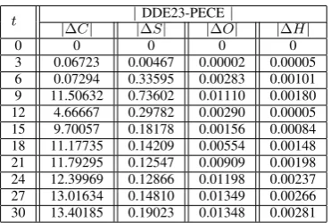
Referring to Table (II), it can be noticed that the dif-ferences of the numerical results obtained utilizing the two methods are quite large on the coconut yieldC(t). This can be overcome by reducing the step sizehof the PECE method from h = 0.01 to h = 0.001. The numerical simulation consequently results in reducing the size of discrepancy as shown in Table III. Hence, reducing the step size h of the PECE method has a great impact on the accuracy of the numerical results.
B. Simulation results of the problem (1)-(2) forα= 0.9
[image:5.595.51.291.536.780.2]0 200 400 600 800 1000 1200 1400 C(t)
0 20 40 60 80 100
S(t)
(a)
0 20 40 60 80 100
S(t) 0
5 10 15
O(t)
(b)
0 20 40 60 80 100
S(t) 2
2.5 3 3.5 4
H(t)
[image:6.595.322.522.57.429.2](c)
Fig. 2: Numerical results obtained using the PECE method with α = 1, τ = 0.1, h = 0.01, and the simulation time
T = 30, (a) dynamics betweenC(t)andS(t), (b) dynamics between S(t) and O(t), (c) dynamics between S(t) and
[image:6.595.64.268.81.460.2]H(t).
TABLE III: Discrepancy of the numerical results of the problem (1)–(2) for α = 1, τ = 0.1 obtained using the DDE23 solver and the PECE method (h= 0.001).
t | |DDE23-PECE|
∆C| |∆S| |∆O| |∆H|
0 0 0 0 0
3 0.06723 0.00467 0.00002 0.00005 6 0.07294 0.33595 0.00283 0.00101 9 11.50632 0.73602 0.01110 0.00180 12 4.66667 0.29782 0.00290 0.00005 15 9.70057 0.18178 0.00156 0.00084 18 11.17735 0.14209 0.00554 0.00148 21 11.79295 0.12547 0.00909 0.00198 24 12.39969 0.12866 0.01198 0.00237 27 13.01634 0.14810 0.01349 0.00266 30 13.40185 0.19023 0.01348 0.00281
0 200 400 600 800 1000 1200 1400 C(t)
0 20 40 60 80 100
S(t)
(a)
0 20 40 60 80 100
S(t) 0
5 10 15
O(t)
(b)
0 20 40 60 80 100
S(t) 2
2.5 3 3.5 4
H(t)
[image:6.595.320.523.538.664.2](c)
Fig. 3: Numerical results obtained using the PECE method with α = 1, τ = 0.1, h = 0.01, and the simulation time
T = 200, (a) dynamics betweenC(t)andS(t), (b) dynamics between S(t) and O(t), (c) dynamics between S(t) and
H(t).
TABLE IV: Numerical results of the problem (1)–(2) for
α= 0.9, τ = 0.1 using the PECE method withh= 0.001.
t | PECE
∆C| |∆S| |∆O| |∆H|
0 500 20 2 2
3 173.23355 12.97739 9.41423 2.58536 6 311.95077 19.82819 11.22206 2.72312 9 357.43848 22.61053 11.48103 2.86142 12 361.10604 23.71782 11.57423 2.98823 15 360.45823 23.93775 11.61876 3.09766 18 361.54209 23.92124 11.64126 3.19126 21 363.34415 23.88780 11.65437 3.27187 24 365.05575 23.86833 11.66327 3.34179 27 366.50416 23.85648 11.66990 3.40275 30 367.72692 23.84725 11.67505 3.45609
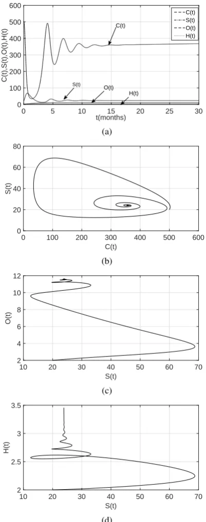
the problem (1)-(2) forα= 0.9, we obtain the approximate solutions as portrayed in Fig4 and the numerical results at some specified timest are shown in Table (IV).
V. CONCLUSIONS
[image:6.595.76.262.631.756.2]0 5 10 15 20 25 30 t(months)
0 100 200 300 400 500 600
C(t),S(t),O(t),H(t)
C(t) S(t) O(t) H(t) C(t)
O(t) H(t)
S(t)
(a)
0 100 200 300 400 500 600
C(t) 0
20 40 60 80
S(t)
(b)
10 20 30 40 50 60 70
S(t) 2
4 6 8 10 12
O(t)
(c)
10 20 30 40 50 60 70
S(t) 2
2.5 3 3.5
H(t)
[image:7.595.65.266.57.567.2](d)
Fig. 4: Numerical results obtained using the PECE method withα= 0.9, τ = 0.1, h= 0.001, and the simulation time
T = 30, (a) numerical solutionsC(t), S(t), O(t), H(t), (b) dynamics betweenC(t)andS(t), (c) dynamics betweenS(t)
andO(t), (d) dynamics betweenS(t)andH(t).
solution for benefit of developing the computation technique based on PECE method to approximate solution for fractional order. The comparison show that PECE method can approx-imate solution close to what approxapprox-imated by ODE 45 and DDE 23, especially when step size is small, in the integer order case both for the model that impose and don’t impose the time delay. Refer to the conformity of approximation from ODE 45, DDE 23, and PECE method, we thus adjust the computation detail of PECE method for approximating the solution of fractional order.
ACKNOWLEDGMENT
This research is supported by the Centre of Excellence in Mathematics, the Commission on Higher Education, Thai-land. This work is also supported by the Department of Mathematics, King Mongkut’s University of Technology North Bangkok, Thailand.
REFERENCES
[1] D. Manna, A. Maiti, and G. Samanta, “Analysis of a predator-prey model for exploited fish populations with schooling behavior,”Applied Mathematics and Computation, vol. 317, pp. 35–48, 2018.
[2] S. G. Mortoja, P. Panja, and S. K. Mondal, “Dynamics of a predator-prey model with stage-structure on both species and anti-predator behavior,”Informatics in Medicine Unlocked, 2017.
[3] K. Belkhodja, A. Moussaoui, and M. A. Alaoui, “Optimal harvesting and stability for a prey–predator model,” Nonlinear Analysis: Real World Applications, vol. 39, pp. 321–336, 2018.
[4] S. Boonrangsiman, K. Bunwong, and E. J. Moore, “A bifurcation path to chaos in a time-delay fisheries predator–prey model with prey consumption by immature and mature predators,”Mathematics and Computers in Simulation, vol. 124, pp. 16–29, 2016.
[5] B. Sahoo and S. Poria, “Effects of additional food in a delayed predator–prey model,”Mathematical biosciences, vol. 261, pp. 62–73, 2015.
[6] C. Liu, Q. Zhang, J. Li, and W. Yue, “Stability analysis in a delayed prey–predator-resource model with harvest effort and stage structure,”
Applied Mathematics and Computation, vol. 238, pp. 177–192, 2014. [7] W. Liu and Y. Jiang, “Bifurcation of a delayed gause predator-prey model with michaelis-menten type harvesting,”Journal of theoretical biology, vol. 438, pp. 116–132, 2018.
[8] S. Rana, S. Bhattacharya, J. Pal, G. M. NGu´er´ekata, and J. Chattopad-hyay, “Paradox of enrichment: A fractional differential approach with memory,”Physica A: Statistical Mechanics and its Applications, vol. 392, no. 17, pp. 3610–3621, 2013.
[9] M. Javidi and N. Nyamoradi, “Dynamic analysis of a fractional or-der prey–predator interaction with harvesting,”Applied mathematical modelling, vol. 37, no. 20, pp. 8946–8956, 2013.
[10] R. K. Ghaziani, J. Alidousti, and A. B. Eshkaftaki, “Stability and dynamics of a fractional order leslie–gower prey–predator model,”
Applied Mathematical Modelling, vol. 40, no. 3, pp. 2075–2086, 2016. [11] I. Podlubny, Fractional differential equations: an introduction to fractional derivatives, fractional differential equations, to methods of their solution and some of their applications. Academic press, 1998, vol. 198.
[12] S. Bhalekar and V. Daftardar-Gejji, “A predictor-corrector scheme for solving nonlinear delay differential equations of fractional order,”
Journal of Fractional Calculus and Applications, vol. 1, no. 5, pp. 1–9, 2011.
[13] K. Diethelm, N. J. Ford, and A. D. Freed, “A predictor-corrector ap-proach for the numerical solution of fractional differential equations,”
Nonlinear Dynamics, vol. 29, no. 1, pp. 3–22, 2002.
[14] K. Diethelm and N. J. Ford, “Analysis of fractional differential equations,”Journal of Mathematical Analysis and Applications, vol. 265, no. 2, pp. 229–248, 2002.