The impact of monetary policy on gold price dynamics
Yanhui Zhu
University of West England
Jingwen Fan
Nottingham Trent University
Jon Tucker
University of West England
Abstract
Ever since the collapse of the Bretton-Woods system, gold has retained its function as an important monetary commodity (Baur and Lucey, 2010), and continues to provide important inflation forecasting information to monetary policy setters (Tkacz, 2007). However, Capie et al. (2005) highlight the instability of gold price dynamics through time, attributing it to unpredictable political attitudes and events. In this paper, we investigate gold price dynamics under different inflation regimes and stock market conditions using UK and US index-linked Treasury bond data. We show that gold lost its role as an inflation hedge after May 1997 in the UK, and after 2003 did not act as an inflation hedge in the US, supporting the argument that gold is an inflation hedge only in periods of high inflation and inflation expectations. Further, we show that gold retained its safe haven status throughout the sample period in both countries, but it did not act as a stock market hedge in the UK except during the 2008-9 global financial crisis. Finally, we conduct an event-study analysis of the impact of QE announcements from four leading central banks on the gold price in US dollars. While the QE announcements of the US Federal Reserve and the European Central Bank exerted a strong and weak influence on gold, respectively, the Bank of England and the Bank of Japan’s QE announcements had no discernible impact on the gold price.
Keywords: Gold price; Hedging; Central banks; Bank of England independence; Quantitative Easing
2
The impact of monetary policy on gold price dynamics
Abstract
3
The impact of monetary policy on gold price dynamics
1. Introduction
The global financial crisis of 2007-8 presented many investors with a strong motivation to search for ‘safe haven’ assets. Since the beginning of 2016, the gold price has risen by more
than 30%, placing it as one of the best performing assets for investors during that period. Conventional wisdom suggests that the gold price and the general price level move together, and as a result for millennia and across cultures gold represented an effective store of value.
Even in the post-Bretton-Woods system era, gold remains an effective investment tool in many countries in the form of coin, bullion, certificates or warrants (Worthington and Pahlavani,
2007). Perusal of the academic literature on gold indicates that of the key economic drivers of the demand for gold, the rate of inflation is the most heavily researched. Fisher (1930) establishes the fundamental positive relationship between expected asset returns and expected
inflation. There is an extensive empirical literature on the relationship between gold prices and inflation, commencing with Jastram (1978), and later extended by Jastram and Leyland (2009),
who examines the long run relationship between the price of gold and inflation in England over the period 1560-2007 and in the US over the period 1808-2007. They find that gold maintained its purchasing power over long periods of time, for example, over 50-year intervals, but was a
poor hedge against major inflation because the purchasing power of gold mirrored that of the general price level under the Gold Standard where the nominal price of gold was held constant.
More recent studies confirm that gold can serve as a profitable investment opportunity under extreme market conditions (see Baur and McDermott, 2010; Narayan et al., 2013; and Narayan
et al., 2015).
4
US setting over the period 2003-2015. Furthermore we investigate the impact of Quantitative Easing (QE) announcements made by the central banks of four major economies on gold prices.
Our paper makes three important contributions. First, we test our hypotheses using market-implied inflation expectations data. Consistent with the recent literature, the data we employ
includes the break-even inflation rate (BEIR), also referred to as inflation compensation, which is the sum of inflation expectations, the inflation risk premium and the liquidity premium. Liu
et al. (2015) argue that the BEIR is increasingly used in central bank publications, market
commentaries and empirical research as it provides the timeliest indicator of inflation expectations (Joyce et al., 2010; Abrahams et al., 2013; and Pflueger and Viceira, 2013). BEIR
may be estimated in real time every trading day without any lag, unlike conventional measures of inflation expectations extracted from economic surveys or forecasted using econometric models, which are available only on a monthly or bi-annual basis. Second, our empirical
models take account of the structural shift in the level of UK inflation and inflation expectations. More specifically, on 6th May 1997, the UK Government handed to the Bank of
England responsibility for the setting of interest rates to meet its stated inflation target. This marked the beginning of the Bank’s operational independence and its full commitment to inflation targeting. We use this event as a cut-off point for the UK sample data as the level of
inflation and inflation expectations are high in the subperiod before this event, and low in the subperiod thereafter. We argue that the changes in the level of inflation and inflation
expectations impact upon the role of gold as an inflation hedge. More precisely, the fall in inflation and inflation expectations should stop the gold price reacting to inflation expectations. When inflation and inflation expectations are at a low level, investors may in this event view
gold as an asset with limited potential in terms of capital gains. Once investors take into account the transaction costs associated with buying and selling gold, they may decide that trading in
5
of Laurent (1994) who argues that the gold price only reacts to changes in ‘deep-seated’ inflation expectations. If investors no longer fear deep-seated inflation then gold should lose
its property as an inflation hedge. Third, we conduct an event study examining the impact of QE-related news announcements on the price of gold. In response to the deterioration of
financial markets during the period 2008 to 2009, the central banks of the major economies embarked upon the unconventional monetary policy of Quantitative Easing (QE). A former Chief Economist of the Bank of England, Spencer Dale, identified the central objective
underlying QE as the injection of a substantial amount of money into the economy via the portfolio rebalancing channel (Dale, 2010). To the extent that investors do not view money as
a perfect substitute for gilts, they will reduce the additional holding of money by switching into other sterling assets or foreign assets, thereby pushing up their prices. There is a large body of literature examining the effect of QE on asset prices (D’Amico and King, 2010; Gagnon et al.,
2011; Krishnamurthy and Vissing-Jorgenson, 2011; Neely, 2011; Joyce et al., 2011; Ugai 2007; and Wright, 2012). Despite differences in the methods and sample periods employed,
the majority of existing studies agree that QE had a significant impact on Treasury yields, though evidence of its effect on other assets such as corporate bonds and equities is mixed. By means of an event study approach, Gagnon et al. (2011) find that the QE1 round of the US
Federal Reserve had a significant and negative impact on the yield of higher-grade corporate bonds and mortgage backed securities (MBS). Using a VAR analysis, Wright (2011) shows
that the monetary policy shock lowered higher-grade corporate bond yields and raised stock prices, with the effects wearing off after a few months. However, Krishnamurthy and Vissing-Jorgensen (2011) demonstrate that the impact of QE1 and QE2 had a smaller effect on
lower-grade corporate bonds, and the impact of QE on MBS was only marked in QE1 where QE involved MBS purchases. Using both event studies and a VAR analysis, Joyce et al. (2011)
6
impact on equities was potentially large but highly uncertain as the announcement of QE may give investors information concerning the outlook of the economy and corporate earnings. If
the outlook is worse than expected then it should lower their expectations for dividend payments, resulting in lower equity prices. To date, no paper has focused attention on the
impact of QE on the gold price. As a store of value, gold provides an alternative to financial assets such as money and gilts. Even if a small proportion of gilts previously held by investors is replaced with gold as a result of QE, the increase in demand should push the gold price higher
simply as a result of the portfolio rebalancing channel. Therefore, we argue that the announcement of the commencement or an expansion of QE should give rise to a positive
impact on the gold price, and an indication of the end or the reduction of QE should produce a negative impact.
Our key results may be summarised as follows. First, gold provided an effective hedge against
inflation over the subperiod of 1985-1997 in the UK when inflation and inflation expectations were high. But it proved not to provide an inflation hedge in the UK over the subperiod of
1997-2015 or in the US over the period of 2003-2015 when inflation and inflation expectations were low. Second, gold acted as a stock market hedge in the US over the period of 2003-2015, but did not provide such a hedge in the UK over either the same period or over the whole
sample period of 1985-2015. However, gold acted as a stock market hedge during the global financial crisis in both countries, and provided a safe haven in all periods examined for both
countries. Third, our results show that gold has provided an effective currency hedge for investors over both the whole study period and the sub-sample periods in the UK, and over the whole study period in the US. Finally, using an event-study analysis we find evidence of a
significant impact of US Federal Reserve QE announcements on the gold price, while the influence of the European Central Bank QE announcements is much weaker. The gold price
7
of Japan. The rest of our paper is organised as follows. In section 2, we review the academic literature on gold as a hedging tool. In section 3 we discuss the data employed in our study,
followed by the econometric model which we discuss in section 4. In section 5, we present and discuss the empirical evidence arising from our models. Section 6 provides a summary and
conclusion.
2. The gold price and its determinants
Generally speaking, there are two main reasons for people to hold gold: (i) for the purposes of consumption e.g. for jewellery; (ii) for the purposes of investment or preserving wealth,
whereby gold is used to hedge against inflation, exchange rate and stock market fluctuations. Laurent (1994) argues that the stable purchasing power of gold was instrumental to the automatic price stabilisation mechanism of the Gold Standard (see also Mill, 1987 and Barro,
1979). Under the Gold Standard, a rise of the price level of goods relative to that of gold meant a fall in the purchasing power of gold. This reduced the incentive to produce gold and diverted
some of the existing gold stock from monetary to consumption uses such as jewellery, thereby causing the money supply to fall. The fall in the money supply caused the price level of goods to fall until the relative price of gold rose to its long-term level. Conversely, a fall in the general
price level relative to gold encouraged gold producers to find and extract new gold at a greater cost, causing the money supply and the price level of goods to rise.
However, under a system of fiat money, there is no longer a built-in stabilisation mechanism, and thus gold becomes a commodity like any other. Garner (1995) argues that whether the price of gold relative to the general price level remains stable depends on different forces. A rise in
inflation expectations may cause investors to shift their funds from financial assets, such as money and bonds, to gold. As the supply of gold is more or less fixed in the short run, even a
8
price level rises gradually because the price of many goods and services adjusts only slowly. As a result, the rise in the gold price might precede a rise in general prices provided that
inflation expectations are correct. Thus, the relative price of gold should still be stable in the long run, while it should also act as a leading indicator for inflation.
The empirical evidence in general shows that the nominal price of gold and the general price level move together in the long run. Herbst (1983) and Laurent (1994) study the gold price and the wholesale price index in the US and find that the two series moved closely over the last two
centuries and the real price of gold on average remained constant, even though the price of gold was pegged for substantial periods and the wholesale price increased dramatically during that
time. In a study of the aftermath of the collapse of the Bretton Woods system, Beckmann and Czudaj (2013) find that the price of gold and the general price level are cointegrated in the US, the UK, Japan and the Euro area, indicating that a long-term stable linear relationship existed
in the period from 1970 to 2011. Worthington and Pahlavani (2007) find evidence of cointegration for the US after allowing for endogenous structural breaks in the post-war period.
Using a threshold cointegration technique, Wang et al. (2011) show that the price of gold and the general price level are characterised by a linear cointegrated relationship for the US, while for Japan there is a threshold cointegrated relationship.
However, empirical evidence on the relationship between inflation and gold returns in the short run is somewhat inconclusive. Chua and Woodward (1982) show that actual, expected and
unexpected inflation rates are significant explanatory factors for gold returns over the period 1975 to 1980 for the US, though not for Canada, Germany, Japan, Switzerland and the UK. Jaffe (1989) finds for the US that gold returns are significantly related to actual, but not
expected, inflation over the period 1971 to 1987. Laurent (1994) and Garner (1995) find that lagged gold returns can explain the inflation rate, but the predictive power of such returns is
9
measure economic slack such as the unemployment rate and the manufacturing capacity utilization rate. Mahdavi and Zhou (1997) employ an out-of-sample forecast method and find
that gold returns are the worst predictor compared to a general commodity price index and the past inflation rate. Cecchetti et al. (2000) use a similar method and find that gold prices can
improve the forecast accuracy of the rate of inflation. However, they find that an increase in gold prices preceding future declines in inflation appears counterintuitive, questioning the use of gold as a predictor of inflation. Examining the intraday price of gold futures, Cai et al. (2001)
and Christie-David et al. (2000) find that the release of monthly inflation data increases the volatility of gold futures. However, using daily data, Blose (2010) shows that announcement
day inflation surprise has no impact on gold returns in the US over the period 1988 to 2008. Erb and Harvey (2013) measure unexpected inflation simply by taking the difference between the inflation rate in any period and that of the previous period, and find little evidence that gold
was an effective hedge against unexpected inflation in the US over the period 1975 to 2011. However, Tkacz (2007) finds that the return on gold predicts the rate of inflation over a 12-18
month horizon in most developed countries which have formal inflation targeting over the period 1995 to 2004. He argues that in those countries, inflation expectations are more accurate and thus gold returns are more likely to predict inflation accurately.
In relation to the role of gold as a currency hedge, Sjaastad and Scacciavillani (1996) argue that an appreciation in a local currency can cause the price of gold in that currency to fall. Capie
et al. (2005) find evidence for such a negative relationship between the US dollar gold price
and the value of US dollars against the yen and sterling over the period 1971 to 2004. However, they find that the strength of this relationship varies over time and was much weaker before
1976 and after 1985. Pukthuanthong and Roll (2011) confirm the negative relationship between a given currency and the gold price denominated in that currency for the yen, euro and sterling
10
the residuals. Using copulas to examine the role of gold as a safe haven or hedge against the US dollar, Reboredo (2013) find significant positive average dependence and symmetric tail
dependence between gold returns in six currencies and US dollar depreciation against these currencies over the period 2000 to 2012, indicating that gold can act as a hedge and a safe
haven against currency movements. Using quantile regressions, Ciner et al. (2013) show that over the period from 1990 and 2010, gold acted as a safe haven investment against exchange rate movements in both the US and UK.
It is also widely held that gold can act as a stock and bond market hedge in normal market conditions, and a safe haven in ‘abnormal’ times, thereby providing diversification benefits to
portfolio holders. Hillier et al. (2006) show in a study of the US that gold has a small negative beta in normal market conditions and a larger negative beta in volatile market conditions. Baur and McDermott (2010) conduct an extensive study for 13 countries over the period 1979 to
2009, and find that gold provides both a hedge and a safe haven for stock investors in most developed countries, while the safe haven effect in emerging countries is weaker. Using
wavelet analysis, Bredin et al. (2015) find that gold acts as a hedge for a variety of international equity and debt markets for horizons of up to one year. Further they find that gold acted as a safe haven for equity investors around the 1987 ‘Black Monday’ crash and the global financial
crisis. However, Agyei-Ampomah et al. (2014) study a sample of sovereign bonds for 13 countries and show that other precious metals and industrial metals tend to outperform gold as
either hedging vehicles or safe haven assets against losses in sovereign bonds.
3. Data
In this paper we model gold price dynamics against data for inflation expectations, exchange rates and stock market returns. We measure gold prices using the London PM fixing price in
11
expectations calculated by the Bank of England using data from index-linked gilts and conventional gilts for the UK, and for the US we use those calculated by the US Treasury using
Treasury Inflation Protected Securities (TIPS) and conventional Treasury securities. UK ex-ante 5-year and 10-year inflation expectations and real interest rates are estimated using a
spline-based technique (Anderson and Maule, 2014) and the US data are estimated using a quasi-cubic hermite spline function (US Department of Treasury, 2009). For exchange rates, we collect trade-weighted exchange rate data for both the UK pound sterling and the US dollar,
and we compute returns on the FTSE 100 index and the S&P 500 index for stock returns for the UK and US, respectively. For the event-study analysis, we also collect the 3-month
Treasury bill rates for the US and the news releases related to Quantitative Easing of the US Federal Reserves (FED), the European Central Bank (ECB), the Bank of England (BOE) and the Bank of Japan (BOJ). All UK data other than the FTSE 100 index, which is taken from
Datastream, are collected from the Bank of England Statistical Interactive Database. All US data other than the S&P 500 index, which is taken from Datastream, are collected from Federal
Reserve Bank of St. Louis FRED Database. All QE related announcement data are collected from two survey papers (Fawley and Neely, 2013; Agostini et al. 2016). Our data consist of daily observations covering the period 2nd January 1985 to 19th March 2015 for the UK, and
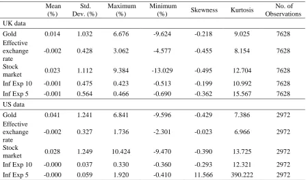
the period 2nd January 2003 to 19th March 2015 for the US. Table 1 reports descriptive statistics for the model variables. Data for gold prices, exchange rates and the stock index are all
transformed to natural log differences to avoid spurious regressions associated with non-stationary variables (Granger and Newbold, 1974). Specifically, our unit root test results suggest that the natural logarithms of these variables are non-stationary, but their first-order
differences are stationary1. 5-year and 10-year inflation expectations are calculated by taking the differences between the expectations on any given day and those on the previous day.
12
We can observe that the FTSE 100 index produces returns which are on average higher and more volatile than gold during the period 1985 to 2015. The average daily return of the FTSE
100 index is 0.023% which is higher than the average return of gold at 0.014%, and the standard deviation of FTSE 100 index daily return is 1.112%, slightly higher than its counterpart for
gold at 1.032%. However, the S&P 500 index produces lower average returns than gold and the two variables have very similar volatility over the period 2003 to 2015. The average daily return of the S&P 500 index is 0.028% which is lower than the average return of gold at 0.041%,
and the standard deviation of the S&P 500 index daily return is 1.249%, similar to its counterpart for gold at 1.241%. The pound sterling and the US dollar both depreciate against
the associated basket of currencies in their respective sample periods by an average of 0.002% per day. All of the model daily returns are insignificantly different from zero and the respective variable distributions exhibit fat tails, with kurtosis values much greater than the value of 3 for
normally distributed variables. The kurtosis of the returns on gold, the exchange rate, and the FTSE 100 index for the UK are 9.025, 8.154 and 12.704, respectively, and for the US they are
7.386, 6.966 and 13.725, respectively. On average, the UK’s 10-year inflation expectations fell by 0.06 basis points per day over the period. This observation is not surprising as the sample commenced in January 1985 when average annual inflation expectations for the following 10
years was 7.44% and ended in March 2015 when average annual inflation expectations for the following 10 years was only 2.69%. On average, the 10-year and 5-year inflation expectations
for the US did not change over the study period. Consistent with the model returns, the daily changes in inflation expectations are insignificantly different from zero. Perhaps as expected, the data on US 5-year inflation expectations have a few outliers around the time of the Lehman
Brothers bankruptcy which give rise to extreme values for skewness and kurtosis.
13
4. Modelling UK and US gold price dynamics
4.1 Regression analysis
Our baseline model is described in Equations 1 and 2 below. Equation 1 models the relation between gold returns and inflation expectations, the exchange rate and stock market returns.
Equation 2 is a GARCH model to take account of conditional heteroskedasticity in the data.
𝑟𝑟𝐺𝐺𝐺𝐺𝐺𝐺𝐺𝐺,𝑡𝑡 = 𝛽𝛽0+ 𝛽𝛽1∆𝜋𝜋𝑝𝑝,𝑡𝑡𝑒𝑒 + 𝛽𝛽2𝑟𝑟𝑒𝑒𝑒𝑒,𝑡𝑡+ 𝛽𝛽3𝑟𝑟𝑚𝑚,𝑡𝑡+ 𝛽𝛽4𝑟𝑟𝑚𝑚(𝑞𝑞),𝑡𝑡+ 𝑢𝑢𝑡𝑡 (1)
ℎ𝑡𝑡 = 𝛾𝛾0+ 𝛾𝛾1(𝑢𝑢𝑡𝑡)2+ 𝛾𝛾2ℎ𝑡𝑡−1 (2)
Note that 𝑟𝑟𝐺𝐺𝐺𝐺𝐺𝐺𝐺𝐺,𝑡𝑡 is the return on sterling or dollar gold prices in period t, ∆𝜋𝜋𝑝𝑝,𝑡𝑡𝑒𝑒 is the change in
the p-year UK or US inflation expectation in period t (where p = 5 or 10), 𝑟𝑟𝑒𝑒𝑒𝑒,𝑡𝑡 is the rate of change of the effective exchange rate of pound sterling or the US dollar in period t, 𝑟𝑟𝑚𝑚,𝑡𝑡 is the return on the FTSE 100 index or the S&P 500 index in period t, and 𝑢𝑢𝑡𝑡 is the error term. Following Baur and Lucey (2010), 𝑟𝑟𝑚𝑚(𝑞𝑞),𝑡𝑡 (q = 1% or 5%) is a multiplicative dummy variable
equal to the market return when the market return is in the q lower quantile; 𝑟𝑟𝑚𝑚(𝑞𝑞),𝑡𝑡 is zero in all other periods. The error term, 𝑢𝑢𝑡𝑡, is assumed to follow a GARCH (1,1) process with a time varying variance, ℎ𝑡𝑡. The GARCH model is used to control for heteroskedasticity in the data which is common in daily financial data.
We formulate four hypotheses in order to determine whether gold can serve as an inflation hedge, exchange rate hedge, stock market hedge, and safe haven asset.
Hypothesis 1a: 𝛽𝛽1> 0 (gold is an inflation hedge in periods of high inflation expectations) Hypothesis 1b: 𝛽𝛽1 = 0 (gold is not an inflation hedge in periods of low inflation expectations) Hypothesis 2: 𝛽𝛽2 < 0 (gold is a currency hedge)
14
𝛽𝛽1 measures the relation between the gold return and the change in inflation expectations. A
positive 𝛽𝛽1 implies that a rise in inflation expectations would see the gold price rising, thereby producing a positive return. This could be caused by investors treating gold as an inflation
hedge and diverting their holdings of financial assets to gold when inflation is expected to rise in the future. The gold price is believed to rise at the same rate as the general price level in the
long term. Thus, when inflation is expected to rise so is the gold price. However, investor attitude towards gold may be dependent on the level of inflation expectations. If inflation expectations are rising from a very low base, investors may feel the gains from switching to
gold are too small to cover transaction costs. However, when they are expecting higher inflation at a time of already high inflation, the perceived gains from switching may be great enough to
warrant a switch. Our UK data cover a long period which includes some years of high inflation (1991:8.40%) and some years of close to zero inflation such as in 2015. Thus our sample provides an ideal setting to test our hypotheses 1a and 1b using subsample data corresponding
to high and low inflation expectations, respectively.
𝛽𝛽2 measures the relation between the gold return and the rate of change in the trade-weighted
exchange rate. For an internationally traded commodity such as gold, a change in any exchange
rate should result in an adjustment in its price denominated in the currency of a country which does not have absolute market power in that commodity (Sjaastad and Scacciavillani 1996). Despite the dominance of London as a trading centre for gold (Lucey et al. 2013), the UK has
little market power in the global gold market (Sjaastad and Scacciavillani 1996; Sjaastad 2008). Furthermore, although the USD currency block has gained market power in the global gold
market this century, its market power is far from absolute (Sjaastad 2008). Thus, as the pound sterling or the US dollar depreciates, the gold price in the respective currency is expected to rise. If Hypothesis 2 is supported, then gold acts as a currency hedge as gold priced in pounds
15
Baur and Lucey (2010, p. 219) defined a hedge as “an asset that is uncorrelated or negatively correlated with another asset or portfolio on average”, and a safe haven asset as “an asset that
is uncorrelated or negatively correlated with another asset or portfolio in times of market stress or turmoil”. The correlation coefficient between the gold return and the FTSE 100 index or the
S&P 500 index return on average is measured by coefficient 𝛽𝛽3. If Hypothesis 3 is supported, then gold acts as a hedge for stock index returns. Finally, the sum of the estimated coefficients
𝛽𝛽3 and 𝛽𝛽4 measures the coefficient between the gold return and the FTSE 100 index return or
the S&P 500 index return when the stock market is in stress. In the baseline model, the market
stress is measured by the 1% lowest quantile dummy. In the alternative parameterization, a 5% quantile dummy is used. If no evidence is found to reject Hypothesis 4, then gold acts as a safe
haven asset.
4.2 Event-study analysis
We examine the impact of Quantitative Easing on gold returns using an event study. We follow
the approach used by Tucker et al. (2013), employing a dummy variable model (see also Thompson (1982) and Salinger (1992) for further discussion). The model is simply obtained
by appending a vector of dummy variables to the conventional Capital Asset Pricing Model (CAPM). Thus, for each news announcement, i, abnormal returns are estimated from the model
represented by equation (3) below:
𝑟𝑟𝐺𝐺𝐺𝐺𝐺𝐺𝐺𝐺,𝑖𝑖,𝑡𝑡− 𝑟𝑟𝑓𝑓,𝑡𝑡 = 𝛾𝛾𝑖𝑖 + 𝜃𝜃𝑖𝑖�𝑟𝑟𝑚𝑚,𝑡𝑡− 𝑟𝑟𝑓𝑓,𝑡𝑡� + ∑27𝜏𝜏=1𝛼𝛼𝑖𝑖,𝜏𝜏𝐷𝐷𝑖𝑖,𝜏𝜏,𝑡𝑡+ 𝜀𝜀𝑖𝑖,𝑡𝑡 (3)
16
period consists of 77 day-observations from 55 days before to 21 days after the announcement. The abnormal returns are estimated for 27 days; 5 days pre-event, 1 day event (announcement
day) plus a further 21 post-event days. For example, 𝐷𝐷𝑖𝑖,1,𝑡𝑡 equals 1 five days before the news announcement, 𝐷𝐷𝑖𝑖,6,𝑡𝑡 equals 1 on the event day, and 𝐷𝐷𝑖𝑖,27,𝑡𝑡 equals 1 on the 21st day of the post-event period.
Hypothesis 5 is formulated to examine the impact of QE announcement on the gold price.
Hypothesis 5a: 𝛼𝛼𝑖𝑖,𝜏𝜏 > 0 (gold price rises when QE is announced to commence or expand) Hypothesis 5b: 𝛼𝛼𝑖𝑖,𝜏𝜏 < 0 (gold price falls when QE is announced to stop or shrink)
Quantitative Easing is one of the unconventional monetary policies widely employed by major central banks after the policy rate hits the zero lower bound. One of the main channels
through which QE may work is the portfolio rebalancing channel. By buying long-term assets such as Treasury bonds and MBS from the private sector, central banks expect investors to
replace them with assets similar in terms of risk and maturity, therefore pushing up the prices of long-term assets in general and bringing down the long-term interest rates which are crucial to consumer and business borrowing decisions. Gold is a store of value and as such
provides investors with an alternative investment tool to financial assets such as long-term Treasury bonds or MBS. Therefore, we argue that any news indicating the commencement or
expansion of QE should be positive for the gold price. Further, any news indicating an end to, or reduction in, QE should be negative for the gold price. As an international asset, gold is demanded by investors across countries, and therefore the gold price may be sensitive to the
QE news from across the major economies’ central banks. We identify 45 unambiguous QE announcements made by the FED (12), ECB (8), BOE (8) and BOJ (17) where central banks released news about their asset purchase programmes rather than their liquidity provision
17
announcement on the gold price on the day of announcement, as well as up to five days before and up to 21 days after the announcement. If hypothesis 5a or 5b is supported, then
gold is affected by Quantitative Easing. If the gold market is efficient, then there should be no leakage or delayed response (post-event correction) to an announcement, and therefore the
abnormal returns for all days apart from the announcement.
5. Empirical results
5.1 Inflation hedge
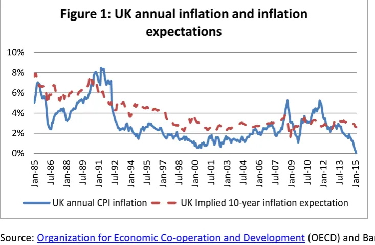
Figure 1 shows the annual percentage change in the UK Consumer Price Index (CPI) and 10-year inflation expectations implied by index-linked gilts and conventional gilts data over the
period 1985 to 2015. Actual and expected inflation are highly correlated and follow a downward trend in this period. After reaching a peak of 8.40% in July 1991, the actual inflation rate fell sharply throughout the early 1990s, and then remained subdued at around 2% until
early 2008. In a 2002 speech, the then governor of Bank of England, Mervyn King, observed that since inflation targeting was introduced in the UK, inflation has been lower, less volatile
and less persistent (King, 2002). Importantly, on 6th May 1997, the UK government granted operational independence to the Bank of England, making it responsible for monetary policy decisions, with the aim of keeping inflation close to the target of 2.5% (reduced to 2% in 2003).
The fall in the level of both inflation and inflation expectations may be partly attributed to an explicit and credible inflation target which helps to anchor the private sector’s views regarding
long-run inflation risk (Gurkaynak, Levin and Swanson, 2010). However, Lin and Ye (2007) argue that inflation targeting has no significant effect on either inflation or inflation variability in seven industrial countries. Whether inflation targeting is the cause of, or simply coincides
with, a period of low and stable inflation in the UK, the moment when it was introduced may serve as a cut-off point in our analysis. The subperiod beforehand features high inflation and
18
is an inflation hedge when inflation and inflation expectations are high. The subperiod afterwards is characterized by low and stable inflation and inflation expectations, and the data
from this subperiod is employed to test hypothesis 1b; gold is not an inflation hedge when inflation and inflation expectations are low.2 In the relatively short sample period for the US
(2003-2015), neither inflation nor inflation expectations experienced dramatic changes. Instead they were low and stable at around 2% during this period, as observed in Figure 2. As a result, the entire sample period for the US is treated as a period of low inflation expectations and is
employed to test hypothesis 1b alone.
[Insert Figures 1 and 2 here]
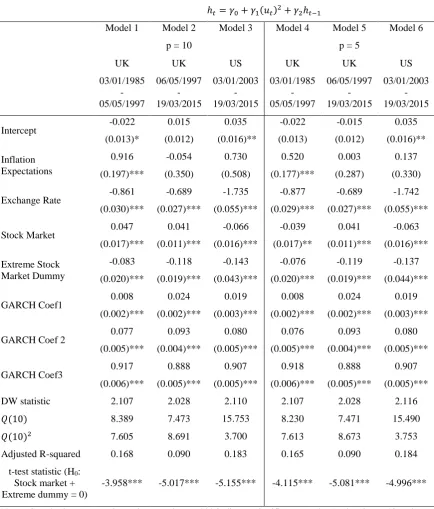
The results of our models for the inflation hedge hypotheses are presented in Table 2. Model 1, which uses UK 10-year inflation expectations, examines the period of high inflation and inflation expectations (1985-1997). The coefficient for inflation expectations is positive at
0.916 and highly significant, indicating that gold acted as an inflation hedge during the subsample period. Thus gold prices rise by 0.916% with a 1% increase in 10-year inflation
expectations. However, this significant positive relationship disappears in the second subsample period of 1997-2015, as shown in Model 2. In effect, gold prices stopped reacting to changes in inflation expectations, suggesting that gold lost its ability to act as an inflation
hedge, and providing some support for hypothesis 1b; investors did not buy gold in the presence of rising inflation expectations when the level of inflation and inflation expectations were low.
Model 3, which uses 10-year inflation expectations for the US, examines the period of low inflation and inflation expectations. Similar to the UK result for the second subsample, the US result gives an insignificant relationship between inflation expectations and gold, providing
further support for hypothesis 1b. Models 4, 5 and 6, where 5-year inflation expectations are
2During the implementation of the Bank of England’s quantitative easing programmes, inflation rose sharply to
19
employed, provide results which are very similar to those for Models 1, 2 and 3 respectively. More specifically, a 1 percent movement in 5-year inflation expectations is associated with a
0.520 percent change in gold prices in the period of high inflation in the UK, 1985-1997, while the coefficient estimates for 5-year inflation expectations are insignificantly different from zero
in the Models 5 and 6, indicating that gold loses its inflation hedge property in the period of low inflation and low inflation expectations. Table 2 also shows the diagnostic test results for each model. There is no evidence of autocorrelation remaining in either the residuals or squared
residuals. The R-squared statistic for the US model (Model 3) is the highest at 0.183, followed by the UK model in the high inflation period (Model 1) at 0.168, and the UK model in the low
inflation period (Model 2) at 0.090. All of the control variables, including the rate of change of effective exchange rate and the stock market and extreme stock market dummies, are highly significant.
[Insert Table 2 here]
5.2 Currency hedge, stock market hedge and safe haven asset
Table 3 summarizes the results for the currency hedge, stock market hedge and safe haven asset. There is a negative relationship between gold returns and movements in the exchange
rate for both UK and US. The results in Model 1 shows that a 1 percent appreciation of the pound against a basket of currencies is associated with a 0.769 percent fall in gold prices over
the period 1985 to 2015. In other words, the elasticity of the gold price to the effective sterling exchange rate is 0.769 for the whole sample. Model 3 shows that the elasticity of the gold price to the effective dollar exchange rate is 1.735 in the shorter and more recent sample period of
2003 to 2015. Model 2 shows the UK results estimated using the data for an identical period to that for the US sample, for the purposes of comparison, and gold price elasticity to the effective
20
z-statistics above 20 in each case. Hence, the evidence presented provides strong support for hypothesis 2; gold acts as a currency hedge in both the UK and US.
[Insert Table 3 here]
The results for the stock market hedge and safe haven vary between the UK and US. When we examine both the full sample and the more recent sample for the UK in Models 1 and 2, respectively, we find a positive and significant relationship between gold returns and stock
returns, suggesting that gold does not act as an effective stock market hedge. Instead, the gold price in sterling moves in the same direction as the stock market on average. In contrast, Model
3 shows a negative and significant relationship between the gold price in dollars and the stock market, suggesting that gold does indeed act as an effective hedge for the US. These results might be explained by a difference in the perspective of UK and US investors. In particular,
UK investors may be more internationally orientated than their US counterparts in their investment decisions. For example, in 2010, UK investors held 50% of their equity portfolio in
foreign stocks, while only 28% of the equity portfolio of US investors was held in foreign stocks (Philips et al., 2012). When domestic stocks are performing badly, UK investors are more likely to switch into international stocks instead of gold. In contrast, US investors may
see their investment options more in terms of stock versus gold.
The F-test for the hypothesis (𝛽𝛽3+ 𝛽𝛽4) = 0 in Model 1 and Model 3 is significant at the 1% level, indicating that gold acted as a safe haven asset for UK investors over the period 1985 to
2015, and for US investors over the period 2003 to 2015, results which are consistent with the findings of Brian and Lucey (2010). In Model 2, the F-test statistic is insignificant, indicating that gold acts as a safe haven over the later subperiod of 2003 and 2015 for the UK as well. To
21
of the global financial crisis is widely considered to be 7th August 2007, when the French bank BNP Paribas suspended redemption of shares held in some of its money market funds (Mishkin,
2011). The end date of crisis is identified as 18th March 2009, when the Fed announced to purchase $300 billion in Treasuries, an additional $100 billion in government-sponsored
enterprise (GSE) debt, and $750 billion in mortgage-backed securities (MBS). Both the FTSE 100 index and the S&P 500 index hit bottom after a more than 40% fall on the previous year several days before this key policy announcement. Model 5 shows the US results during the
crisis period are the same as those for the whole US sample; thus gold acted as a stock market hedge and safe haven asset for US investors during the crisis. More interestingly, Model 4
shows that the stock market coefficient is insignificantly different from zero, indicating that gold is a stock market hedge for UK investors during the crisis period, thereby highlighting its different properties in the wider periods covering both the crisis and normal times. As a
robustness check, we follow Baur and McDermott (2010) and run Models 1 to 5 from Table 3 with a dummy variable capturing the least extreme stock market movements corresponding to
the 5% lowest quantile of the returns distribution. The results of this are shown in table A1 in the appendix and are very similar to the equivalent models where the dummy variable picks up the most extreme stock market movements. Overall, hypotheses 3 and 4 are strongly supported
in the US data, and partly supported in the UK data.
5.3 Quantitative Easing and gold price
The event-study results are presented in four separate tables corresponding to the source of the QE announcement. Table 4 reports the event-study results for the QE announcements made by
22
table along with the estimated abnormal returns of the gold price and the t statistics on the announcement day and up to 3 days before and up to 3 days after the announcement3.
[Insert Table 4]
There are 12 QE announcements by the Fed, of which eight are followed by significant
movements of the gold price in the following day. This may be explained by the fact that our data for the gold price is collected at 15:00 London GMT when the Fed’s policy decision for the day may not have been made. If the news is announced by the Fed at day+0, its impact is
more likely to be observed at day+1. With one exception, all eight significant announcements have the anticipated sign. That is, when the Fed announced a commencement or an expansion of QE, the gold price often rose significantly. For example, on 18th March 2009 the Fed
announced that it would purchase $300 billion in Treasuries, $100 billion in GSE debt and $750 billion in MBS. This was followed by a 6.68% rise in the gold price one day later.
Similarly when the Fed indicated a pause or reduction of QE, gold prices tended to fall significantly. For example, on 18th December 2013, the Fed stated that it would begin tapering and reduce its bond purchases by $10 billion per month from the following January. This was
followed by a 2.77% fall in the gold price on the following day. The results for the pre-event days are insignificant with one exception, indicating little leakage of QE information. However,
there are three cases where the post-event days are significant. In particular, both of the announcements made in 2014 were followed by two days of significant results with anticipated
signs, suggesting that the market became slower in digesting QE related news.
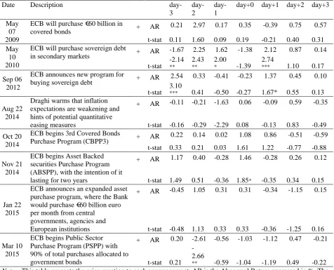
The results of the ECB QE announcements are summarized in Table 5. Compared with other central banks, the ECB was a late-comer in implementing QE policy. This can be seen in the
Table which shows only three QE announcements made before 2014. Out of all eight ECB
23
events, three gave significant and anticipated results. The result for the 10th May 2010 announcement is quite interesting, with abnormal returns positive and significant for both
pre-event and post-pre-event days. These results suggest that the market anticipated that the ECB would come up with a buying strategy as Greece officially requested a bailout on the 23rd April 2010,
together with its credit rating being downgraded to BB+ on 27th April that year.
[Insert Table 5]
The event-study results for the Bank of England (BOE) and the Bank of Japan (BOJ) are
presented in Tables A2 and A3 in the appendix. None of the eight QE announcements of the BOE produced any significant results on the announcement days or one day later. Two of the 17 QE events of the BOJ gave significant results on the announcement day4, but the signs were
different from expectations. Overall, the event-study analysis provides strong evidence on the impact of the Fed’s QE announcement on the gold price and weak evidence on the impact of
the ECB, but evidently there is little impact of the BOE and BOJ announcements.
6. Conclusion
This paper tests the hypothesis that gold acts as an inflation, currency and stock market hedge, while providing a stock market safe haven for UK investors over the period 1985 to 2015, and
for US investors over the period 2003 to 2015. We confirm that gold is a good inflation hedge investment instrument over the subsample period of 1985 to 1997 where both inflation and
inflation expectations were high in the UK. However, gold did not provide an inflation hedge in the period of low inflation and inflation expectations in either the UK (1997-2015) or the US (2003-2015). Further, whereas gold acted as a safe haven asset and a good currency hedge
4 Because Japan time is nine hours ahead of the UK, the London PM Price should fully reflect Japanese QE
24
in all the periods studied for both the UK and US, it was not a stock market hedge across periods, except for the crisis period in the UK. Finally, the gold price moved significantly in
response to the many QE announcements of the US Federal Reserve and several QE announcements of the European Central Bank, supporting the argument that QE affected asset
25
References
Abrahams, M., Adrian, T., Crump, R. and Moench, E. (2013), .Decomposing real and
nominal yield curves., New York Federal Reserve, Staff Report n 570, October 2013. Anderson, G. and Maule, B. (2014), .Assessing the risk to inflation from inflation
expectations., Bank of England Quarterly Bulletin, 54(2), 148.62, available at
www.bankofengland.co.uk/publications/Documents/quarterlybulletin/2014/qb14q204.
pdf.
Baur, D. G. and Lucey, B. M. (2010), .Is Gold a Hedge or a Safe Haven? An Analysis of Stocks, Bonds and Gold., The Financial Review, 45, 217-229.
Baur, D. G. and McDermott, T., K. (2010), .Is gold a safe haven? International evidence., Journal of Banking and Finance, 34, 1886.1898.
Beckmanna, J. and Czudajb, R. (2013), .Gold as an inflation hedge in a time-varying
coefficient framework., North American Journal of Economics and Finance, 24, 208-222.
Berger, H., Haan, J. D. and Eijffinger, S. C. W (2001), Central Bank Independence: An Update of Theory and Evidence, Journal of Economic Surveys 15 (1): 3-40
Blose, L. E. (2010), .Gold prices, cost of carry, and expected inflation., Journal of Economics and Business, 62, 35-47.
Bordo, M.D. and Schwartz, A.J. (1994), .The specie standard as a contingent rule: Some evidence for core and peripheral countries, 1880.1990., NBER Working Paper, No 4860.
Capie, F., Mills, T. C. andWood, G. (2005), .Gold as a hedge against the dollar., Journal of International Financial Markets, Institutions & Money, 15, 343-352.
Cecchetti, S. G., Chu, R. S. and Steindel, C. (2000), .The Unreliability of Inflation Indicators., Current Issues in Economics and Finance, 6(4), 1-6.
Chua, J. and Woodward, R. S. (1982), .Gold as an inflation hedge: a comparative study of six major industrial countries., Journal of Business Finance & Accounting, 9(2), 191-197. Dale, S. (2010) QE — One Year On.” Remarks at the CIMF and MMF Conference on “New
Instruments of Monetary Policy: The Challenges., Cambridge, March 12. D’Amico, S. and King, T. (2010), .Flow and Stock Effects of Large-Scale Treasury
Purchases., Finance and Economics Discussion Series 2010-52, available at http://www.federalreserve.gov/pubs/feds/2010/201052/201052pap.pdf
26
Gagnon, J., Raskin, M., Remache, J. and Sack, B. (2011), .Large-Scale Asset Purchases by the Federal Reserve: Did They Work?., Economic Policy Review, 17(1), 41.59. Garner, C. A. (1995), .How useful are leading indicators of inflation?., Economic Review, 2,
1-18.
Granger, C. and Newbold, P. (1974), Spurious regressions in econometrics, Journal of Econometrics, 2, 111-120
Hillier, D., Draper, P. and Fa¤, R. (2006), .Do Precious Metals Shine? An Investment Perspective., Financial Analysts Journal, 62(2), 98-106.
Jaffe, J. F. (1989), .Gold and Gold Stocks as Investments for Institutional Portfolios., Financial Analysts Journal, 45(2), 53-59.
Jastram, R. (1978), .The golden constant: The English and American experience 1560.1976., New York: John Wiley & Sons.
Jastram, R. and Leyland, J. (2009), .The golden constant: The English and American experience1560.2007., London: Edward Elgar Publishing Ltd.
Joyce, M., Lildholdt, P. and Sorensen, S. (2010), .Extracting inflation expectations and inflation risk premia from the term structure: a joint model of the UK nominal and real yield curves., Journal of Banking and Finance, 34, 281.294.
Joyce, M., Lasaosa, A., Stevens I. and Tong, M. (2011), The Financial Market Impact of Quantitative Easing in the United Kingdom., International Journal of Central Banking, 7(3), 113-161.
Joyce, M., Liu, Z. and Tonks, I. (2014). Institutional investor portfolio allocation, quantitative easing and the global financial crisis. Bank of England Working Paper No. 510
King, M. (2002), . The Inflation Target Ten Years On., Bank of England Quarterly Bulletin., 42(4): 459–74.
Krishnamurthy, A. and Vissing-Jorgensen, A. (2011), .The Effects of Quantitative Easing on Long-term Interest Rates., NBER Working Paper no. 17555.
Laurent, R. D. (1994), .Is there a role for gold in monetary policy?., Journal of Economic Perspectives, XVII, 2-14
Lin, S. and Ye, H. (2007), . Does Inflation Targeting Really Make a Difference? Evaluating the Treatment Effect of Inflation Targeting in Seven Industrial Countries., Journal of Monetary Economics., 54(8): 2521–33.
27
Lucey, B. M., Larkin, C. and O’Connor, F. A. (2013), .London or New York: where and when does the gold price originate?, Applied Economics Letters 20, 813–817. Mahdavi, S. and Zhou, S. (1997), .Gold and commodity prices as leading indicators of
inflation: Tests of long-run relationship and predictive performance., Journal of Economics and Business, 49(5), 475-489.
Meier, A. (2009), .Panacea, Curse, or Nonevent: Unconventional Monetary Policy in the United Kingdom., IMF Working Paper No.163, available at
https://www.imf.org/external/pubs/ft/wp/2009/wp09163.pdf
Mishkin, F.S. (2011), .Over the cliff: from the subprime to the global financial crisis., Journal of Economic Perspectives, 25 (1), 49–70
Narayan, P., K., Narayan, S. and Sharma, S. S. (2013), .An analysis of commodity markets: what gain for investors?., Journal of Banking and Finance, 37, 3878-3889.
Narayan, P. K., Ahmed, H. A. and Narayan, S. (2015), .Do momentum-based trading strategies work in the commodity futures markets?., Journal of Futures Markets, 35, 868-891.
Neely, C. (2011), .The Large-Scale Asset Purchases Had Large International Effects.. Federal Reserve Bank of St. Louis Working Paper no. 2010-018C, available at
https://research.stlouisfed.org/conferences/qe/Neely_._2010-018_1_.pdf
Pflueger, C. and Viceira, L. (2013) .Return predictability in the treasury market: real rates, inflation, and liquidity., Harvard Business School, WP-11-094, September 2013. Philips, C.B., Kinniry, F.M.., and Donaldson, S.J. (2012), . The role of home bias in global
asset allocation decisions, Valley Forge, Pa.: The Vanguard Group.
Rogoff, K. (1985) The Optimal Degree of Commitment to an Intermediate Monetary Target., Quarterly Journal of Economics 100 :1169
Salinger, M. (1992) Standard errors in event studies, Journal of Financial and Quantitative Analysis, 27 (1), 39-53
Sjaastad, L. and Scacciavillani, F. (1996), .The price of gold and the exchange rate., Journal of International Money and Finance, 15(6), 879-897.
Thompson, R. (1985) Conditioning the return-generating process on firm-specific events: a discussion of event study methods, Journal of Financial and Quantitative Analysis, 20 (2), 151-168
Tkacz, G. (2007), .Gold Prices and Inflation., Bank of Canada Working Paper no.35 Tucker, J., Guermat, C. and Prasert, S. (2013) Short run reaction to news announcements,
28
Ugai, H. (2007), .Effects of the Quantitative Easing Policy: A Survey of Empirical Analyses., Monetary and Economic Studies, 25(1), 1-48.
US Department of Treasury (2009), Treasury Yield Curve Methodology [online], US Department of Treasury, available from https://www.treasury.gov/resource-center/data-chart-center/interest-rates/Pages/yieldmethod.aspx [accessed February 10th, 2017]
Wang, K., Lee, Y. and Thi, T. N. (2011), .Time and place where gold acts as an inflation hedge: An application of long-run and short-run threshold model., Economic Modelling, 28, 806-819.
Worthington, A. C. and Pahlavani, M. (2007), .Gold investment as an inflationary hedge: Cointegration evidence with allowance for endogenous structural breaks., Applied Financial Economics Letters, 3, 259.262.
29
Table 1
Descriptive Statistics
Mean
(%)
Std. Dev. (%)
Maximum (%)
Minimum
(%) Skewness Kurtosis
No. of Observations UK data
Gold 0.014 1.032 6.676 -9.624 -0.218 9.025 7628
Effective exchange rate
-0.002 0.428 3.062 -4.577 -0.455 8.154 7628
Stock
market 0.023 1.112 9.384 -13.029 -0.495 12.704 7628
Inf Exp 10 -0.001 0.475 0.423 -0.513 -0.199 10.992 7628
Inf Exp 5 -0.001 0.564 0.466 -0.690 -0.362 15.567 7628
US data
Gold 0.041 1.241 6.841 -9.596 -0.429 7.386 2972
Effective exchange rate
-0.002 0.327 1.736 -2.301 -0.023 6.966 2972
Stock
market 0.028 1.249 10.424 -9.470 -0.390 13.725 2972
Inf Exp 10 -0.000 0.037 0.330 -0.360 -0.293 12.321 2972
Inf Exp 5 -0.000 0.059 1.920 -0.410 11.566 390.222 2972
Notes: Gold denotes the daily return of the gold price denominated in £ for the UK and $ for the US. Effective exchange rate denotes the daily rate of change of the trade-weighted exchange rate of the £ for the UK and the $ for the US. Stock market denotes the daily return of the FTSE 100 index for the UK and the S&P 500 index for the US. Inf Exp 10 and Inf Exp 5 denote the daily change in 10-year and 5-year inflation expectations,
30
Table 2
Inflation hedge results
Estimated Equations
𝑟𝑟𝐺𝐺𝐺𝐺𝐺𝐺𝐺𝐺,𝑡𝑡= 𝛽𝛽0+ 𝛽𝛽1∆𝜋𝜋𝑝𝑝,𝑡𝑡𝑒𝑒 + 𝛽𝛽2𝑟𝑟𝑒𝑒𝑒𝑒,𝑡𝑡+ +𝛽𝛽3𝑟𝑟𝑚𝑚,𝑡𝑡
+ 𝛽𝛽4𝑟𝑟𝑚𝑚(1%),𝑡𝑡+ 𝑢𝑢𝑡𝑡
ℎ𝑡𝑡= 𝛾𝛾0+ 𝛾𝛾1(𝑢𝑢𝑡𝑡)2+ 𝛾𝛾2ℎ𝑡𝑡−1
Model 1 Model 2 Model 3 Model 4 Model 5 Model 6
p = 10 p = 5
UK 03/01/1985 -05/05/1997 UK 06/05/1997 -19/03/2015 US 03/01/2003 -19/03/2015 UK 03/01/1985 -05/05/1997 UK 06/05/1997 -19/03/2015 US 03/01/2003 -19/03/2015 Intercept -0.022 (0.013)* 0.015 (0.012) 0.035 (0.016)** -0.022 (0.013) -0.015 (0.012) 0.035 (0.016)** Inflation Expectations 0.916 (0.197)*** -0.054 (0.350) 0.730 (0.508) 0.520 (0.177)*** 0.003 (0.287) 0.137 (0.330) Exchange Rate -0.861 (0.030)*** -0.689 (0.027)*** -1.735 (0.055)*** -0.877 (0.029)*** -0.689 (0.027)*** -1.742 (0.055)***
Stock Market 0.047
(0.017)*** 0.041 (0.011)*** -0.066 (0.016)*** -0.039 (0.017)** 0.041 (0.011)*** -0.063 (0.016)*** Extreme Stock Market Dummy -0.083 (0.020)*** -0.118 (0.019)*** -0.143 (0.043)*** -0.076 (0.020)*** -0.119 (0.019)*** -0.137 (0.044)***
GARCH Coef1 0.008
(0.002)*** 0.024 (0.002)*** 0.019 (0.003)*** 0.008 (0.002)*** 0.024 (0.002)*** 0.019 (0.003)***
GARCH Coef 2 0.077
(0.005)*** 0.093 (0.004)*** 0.080 (0.005)*** 0.076 (0.005)*** 0.093 (0.004)*** 0.080 (0.005)***
GARCH Coef3 0.917
(0.006)*** 0.888 (0.005)*** 0.907 (0.005)*** 0.918 (0.006)*** 0.888 (0.005)*** 0.907 (0.005)***
DW statistic 2.107 2.028 2.110 2.107 2.028 2.116
𝑄𝑄(10) 8.389 7.473 15.753 8.230 7.471 15.490
𝑄𝑄(10)2 7.605 8.691 3.700 7.613 8.673 3.753
Adjusted R-squared 0.168 0.090 0.183 0.165 0.090 0.184
t-test statistic (H0:
Stock market + Extreme dummy = 0)
-3.958*** -5.017*** -5.155*** -4.115*** -5.081*** -4.996***
Notes: Standard errors are shown in parentheses. *** indicates significance at the 1% level. p = 10 and p = 5 denote 10-year and 5-year inflation expectations, respectively. Q(10) and Q(10)2 are test statistics for
31
Table 3
Currency hedge, stock market hedge and safe haven results
Estimated Equations
𝑟𝑟𝐺𝐺𝐺𝐺𝐺𝐺𝐺𝐺,𝑡𝑡= 𝛽𝛽0+ 𝛽𝛽1∆𝜋𝜋10,𝑡𝑡𝑒𝑒 + 𝛽𝛽2𝑟𝑟𝑒𝑒𝑒𝑒,𝑡𝑡+ +𝛽𝛽3𝑟𝑟𝑚𝑚,𝑡𝑡
+ 𝛽𝛽4𝑟𝑟𝑚𝑚(1%),𝑡𝑡+ 𝑢𝑢𝑡𝑡
ℎ𝑡𝑡= 𝛾𝛾0+ 𝛾𝛾1(𝑢𝑢𝑡𝑡)2+ 𝛾𝛾2ℎ𝑡𝑡−1
Model 1 Model 2 Model 3 Model 4 Model 5
UK 03/01/1985 -19/03/2015 UK 03/01/2003 -19/03/2015 US 03/01/2003 -19/03/2015 UK 07/08/2007 -18/03/2009 US 07/08/2007 -18/03/2009
Intercept -0.002
(0.009) 0.036 (0.015)** 0.034 (0.017)** 0.099 (0.070) 0.090 (0.075) Inflation Expectations 0.783 (0.153)*** -0.695 (0.531) 0.716 (0.509) 0.715 (1.867) -0.624 (1.881)
Exchange Rate -0.769
(0.020)*** -0.731 (0.034)*** -1.735 (0.055)*** -0.801 (0.105)*** -2.237 (0.220)***
Stock Market 0.037
(0.009)*** 0.050 (0.015)*** -0.068 (0.019)*** -0.030 (0.040) -0.140 (0.049)*** Extreme Stock Market Dummy -0.093 (0.012)*** -0.068 (0.041)* -0.029 (0.031) -0.032 (0.070) 0.035 (0.080)
GARCH Coef1 0.017
(0.001)*** 0.011 (0.002)*** 0.019 (0.003)*** 0.015 (0.010) 0.011 (0.012)
GARCH Coef 2 0.087
(0.003)*** 0.076 (0.004)*** 0.080 (0.005)*** 0.037 (0.010)*** 0.059 (0.015)***
GARCH Coef3 0.899
(0.004)*** 0.919 (0.004)*** 0.907 (0.005)*** 0.962 (0.011)*** 0.945 (0.016)***
DW statistic 2.056 2.013 2.110 2.067 2.262
𝑄𝑄(10) 5.498 10.783 14.995 5.488 16.297
𝑄𝑄(10)2 9.674 4.640 3.554 9.043 14.040
Adjusted R-squared 0.116 0.089 0.180 0.117 0.128
t-test statistic (H0:
Stock market + Extreme dummy = 0)
-7.735*** -0.480 -4.079*** -1.004 -1.866*
32
Table 4
Federal Reserve QE announcements and gold abnormal returns
Date Description
day-3
day-2
day-1
day+0 day+1 day+2 day+3
Nov 25 2008
FED will purchase $100 billion in GSE Debt and $500 billion in MBS
+ AR -4.06 6.21 7.42 0.20 -0.05 0.52 0.56
t-stat -1.40 2.13
**
2.54
**
0.07 -0.02 0.18 0.20
Mar 18 2009
Fed will purchase $300 billion in Treasuries, additional $100 billion in GSE debt, and $750 billion in MBS
+ AR 0.35 -0.98 -0.13 -2.27 6.68 -0.50 0.20
t-stat 0.21 -0.57 -0.07 -1.31 3.89
***
-0.29 0.11
Nov 03 2010
Fed will purchase additional $600 billion in Treasuries
+ AR 0.84 0.42 -0.46 -0.58 2.33 0.87 -0.64
t-stat 1.10 0.54 -0.60 -0.76 2.95
***
1.13 -0.84
Sep 21 2011
Fed will purchase additional $400 billion in long-term Treasuries while selling equivalent in short-term treasuries
+ AR 0.49 -0.54 -0.07 -1.33 -5.10 -2.11 -5.32
t-stat 0.30 -0.33 -0.04 -0.81 -3.09
***
-1.30 -3.24
***
Jun 20 2012
Fed extends purchase of long bonds/sales of short bonds
+ AR 0.81 -0.67 0.59 -1.43 -0.88 -1.05 0.53
t-stat 0.64 -0.53 0.46 -1.13 -0.67 -0.83 0.41
Sep 13 2012
Fed will purchase $40 billion MBS/month
+ AR 0.42 0.04 -0.18 -1.05 2.13 -0.26 -0.06
t-stat 0.48 0.04 -0.20 -1.16 2.44
**
-0.30 -0.07
Dec 12 2012
Fed will continue to purchase $45 billion in long-term Treasuries per month but without the sale of short-term Treasuries to sterilize purchase
+ AR 0.46 0.72 -0.16 0.44 -1.21 0.35 -0.13
t-stat 0.58 0.90 -0.20 0.55 -1.50 0.43 -0.15
May 22 2013
Bernanke repeats to Congress the Fed is prepared to trim bonds buying if the economy improves sufficiently
- AR -1.41 -0.67 0.61 4.42 -1.47 1.05 0.31
t-stat -0.89 -0.42 0.39 2.77
***
-0.93 0.67 0.19
Jun 19 2013
Bernanke again hints that QE3 could come to an end
- AR 1.13 -0.59 -1.45 1.60 -4.18 0.38 0.40
t-stat 0.63 -0.33 -0.81 0.87 -2.14
**
0.21 0.22
Dec 18 2013
FOMC states that beginning January, it will begin tapering and reduce $10 billion off monthly bond purchases
- AR 0.63 0.28 -0.16 -0.09 -2.77 0.00 0.37
t-stat 0.53 0.23 -0.13 -0.07 -2.34
**
0.00 0.31
Jun 18 2014
Fed announces that QE3 should be finalized by end of October 2014
+ AR 0.72 0.30 -0.58 0.52 1.88 1.58 0.08
t-stat 1.05 0.44 -0.86 0.76 2.75
*** 2.31 ** 0.12 Oct 29 2014
Fed votes to end bond-buying program and announces it will keep rates low
- AR 0.20 -0.24 0.31 -0.39 -1.59 -2.93 0.40
t-stat 0.31 -0.39 0.47 -0.61 -2.49
**
-4.54
***
0.63
33
Table 5
ECB QE announcements and gold abnormal returns
Date Description
day-3
day-2
day-1
day+0 day+1 day+2 day+3
May 07 2009
ECB will purchase €60 billion in
covered bonds + AR
0.21 2.97 0.17 0.35 -0.39 0.75 0.57
t-stat 0.11 1.60 0.09 0.19 -0.21 0.40 0.31
May 10 2010
ECB will purchase sovereign debt
in secondary markets + AR
-1.67 2.25 1.62 -1.38 2.12 0.87 0.14
t-stat -2.14 ** 2.43 ** 2.00 * -1.39 2.74
*** 1.10 0.17
Sep 06 2012
ECB announces new program for
buying sovereign debt + AR
2.54 0.33 -0.41 -0.23 1.37 0.45 0.10
t-stat 3.10
*** 0.41 -0.50 -0.27 1.67* 0.55 0.13
Aug 22 2014
Draghi warms that inflation expectations are weakening and hints of potential quantitative easing measures
+ AR -0.11 -0.21 -1.63 0.06 -0.09 0.59 -0.35
t-stat -0.16 -0.29 -2.29 0.08 -0.13 0.83 -0.49
Oct 20 2014
ECB begins 3rd Covered Bonds
Purchase Program (CBPP3) + AR
0.22 0.14 0.02 1.08 0.86 -0.51 -0.59
t-stat 0.33 0.21 0.03 1.61 1.22 -0.77 -0.88
Nov 21 2014
ECB begins Asset Backed securities Purchase Program (ABSPP), with the intention of it lasting for two years
+ AR 1.17 0.40 -0.28 1.46 -0.28 0.26 0.12
t-stat 1.49 0.51 -0.36 1.85* -0.35 0.34 0.15
Jan 22 2015
ECB announces an expanded asset purchase program, where the Bank would purchase €60 billion euro per month from central
governments, agencies and European institutions
+ AR -0.45 1.05 0.31 0.31 -0.34 -1.15 0.15
t-stat -0.48 1.13 0.33 0.33 -0.36 -1.25 0.16
Mar 10 2015
ECB begins Public Sector Purchase Program (PSPP) with 90% of total purchases allocated to government bonds
+ AR 0.20 -2.61 -0.56 -1.03 -1.12 0.47 -0.21
t-stat 0.21
-2.66
** -0.59 -1.04 -1.19 0.49 -0.22
34
Appendix
Table A1: Currency hedge, stock market hedge and safe haven results (q = 5%)
Estimated Equations 𝑟𝑟𝐺𝐺𝐺𝐺𝐺𝐺𝐺𝐺,𝑡𝑡= 𝛽𝛽0+ 𝛽𝛽1∆𝜋𝜋10,𝑡𝑡
𝑒𝑒 + 𝛽𝛽
2𝑟𝑟𝑒𝑒𝑒𝑒,𝑡𝑡+ +𝛽𝛽3𝑟𝑟𝑚𝑚,𝑡𝑡+ 𝛽𝛽4𝑟𝑟𝑚𝑚(1%),𝑡𝑡+ 𝑢𝑢𝑡𝑡
ℎ𝑡𝑡= 𝛾𝛾0+ 𝛾𝛾1(𝑢𝑢𝑡𝑡)2+ 𝛾𝛾2ℎ𝑡𝑡−1
Model 1 Model 2 Model 3 Model 4 Model 5
UK 03/01/1985 -19/03/2015 UK 03/01/2003 -19/03/2015 US 03/01/2003 -19/03/2015 UK 07/08/2007 -18/03/2009 US 07/08/2007-18/03/2009
Intercept -0.003
(0.009) 0.034 (0.016)** 0.0.035 (0.016)** 0.086 (0.077) 0.065 (0.067)
Inflation Expectation 0.729
(0.151)*** -0.684 (0.530) 0.730 (0.508) 0.803 (1.880) -0.42 (1.745)
Exchange Rate -0.771
(0.020)*** -0.731 (0.034)*** -1.735 (0.055)*** -0.806 (0.103)*** -2.306 (0.223)***
Stock Market 0.032
(0.010)*** 0.052 (0.017)*** -0.066 (0.016)*** -0.018 (0.047) -0.093 (0.037)** Extreme Stock Market Dummy -0.041 (0.013)*** -0.032 (0.029) -0.143 (0.043)*** -0.047 (0.074) -0.194 (0.080)**
GARCH Coef1 0.017
(0.001)*** 0.011 (0.002)*** 0.019 (0.003)*** 0.015 (0.010) 0.013 (0.013)
GARCH Coef 2 0.087
(0.003)*** 0.075 (0.004)*** 0.080 (0.005)*** 0.038 (0.010)*** 0.067 (0.016)***
GARCH Coef3 0.899
(0.004)*** 0.919 (0.004)*** 0.907 (0.005)*** 0.961 (0.012)*** 0.936 (0.017)***
DW statistic 2.059 2.018 2.110 2.073 2.316
𝑄𝑄(10) 4.869 10.108 15.753 5.189 17.069
𝑄𝑄(10)2 9.352 4.661 3.700 9.203 15.708
Adjusted R-squared 0.115 0.086 0.183 0.119 0.121
t-test statistic (H0:
Stock market + Extreme dummy = 0)
-1.221 0.847 -5.155*** -1.177 -3.994***
35
Table A2
Bank of England QE announcements and gold abnormal returns
Date Description day-3
day-2
day-1
day+0 day+1 day+2 day+3
Jan 19 2009 BOE will purchase
up to £50 billion in private assets
+ AR -0.48 -1.74 2.47 -0.41 2.79 -1.34 1.14
t-stat -0.21 -0.76 1.08 -0.18 1.19 -0.58 0.50
Mar 05 2009 BOE announces £75
billion QE program
+ AR -2.36 -2.81 -0.47 -0.25 2.31 -1.64 -1.84
t-stat -1.42 -1.76 -0.29 -0.15 1.44 -1.02 -1.06
May 07 2009 BOE expands QE program to £125 billion
+ AR 0.21 2.97 0.17 0.35 -0.39 0.75 0.57
t-stat 0.11 1.60 0.09 0.19 -0.21 0.40 0.31
Aug 06 2009 BOE expands QE
program to £175 billion
+ AR 1.92 0.07 0.11 0.53 -1.06 -1.04 0.07
t-stat 2.07** 0.07 0.12 0.57 -1.14 -1.13 0.08
Nov 05 2009 BOE expands QE
program to £200 billion
+ AR 1.77 -0.31 2.51 -0.75 0.49 0.17 -0.63
t-stat 1.85* -0.33 2.64 -0.77 0.51 0.17 -0.66
Oct 06 2011 BOE expands QE
program to £275 billion
+ AR 1.57 -0.63 -0.95 1.46 0.86 1.20 0.12
t-stat 0.76 -0.31 -0.46 0.71 0.42 0.58 0.06
Feb 09 2012
BOE expands QE program to £325 billion
+ AR -0.79 0.25 1.22 0.10 -1.72 0.22 0.22
t-stat -0.54 0.17 0.84 0.07 -1.17 0.15 0.15
Jul 05 2012 BOE expands QE
program to £375 billion
+ AR -0.36 1.60 -0.17 -0.46 -0.88 -0.03 0.81
t-stat -0.30 1.33 -0.14 -0.38 -0.73 -0.02 0.68
36
Table A3
Bank of Japan QE announcements and gold abnormal returns
Date Description day-3 day-2 day-1 day+0 day+1 day+2 day+3
Dec 19 2008 BOJ increases monthly JGB purchases to 1.4 trillion/month
AR 1.77 3.76 -1.72 -2.21 1.57 -0.61 0.10
t-stat 0.57 1.24 -0.57 -0.73 0.52 -0.20 0.03
Jan 22 2009
BOJ will purchase up to 3 trillion in commercial paper
AR -0.30 3.03 -1.34 1.28 1.52 3.57 -1.79
t-stat -0.13 1.30 -0.57 0.56 0.67 1.56 -0.78
Feb 19 2009
BOJ will purchase up to 1 trillion in corporate bonds
AR 0.35 1.85 -0.82 1.19 0.36 -1.04 -0.20
t-stat 0.19 0.95 -0.44 0.63 0.19 -0.54 -0.10
Mar 18 2009 BOJ increases monthly JGB purchases to 1.8 trillion/month
AR 0.35 -0.98 -0.13 -2.27 6.68 -0.50 0.20
t-stat 0.21 -0.57 -0.07 -1.31 3.89*** -0.29 0.11
Oct 05 2010 BOJ will purchase 5 trillion in public and private assets
AR -0.24 0.53 -0.43 1.18 1.00 -0.31 -0.43
t-stat -0.33 0.73 -0.59 1.57 1.37 -0.43 -0.59
Mar 14 2011 BOJ will purchase additional 5 trillion in public and private assets
AR 0.26 -1.33 -0.20 0.68 -1.62 0.03 0.05
t-stat 0.29 -1.41 -0.23 0.77 -1.80* 0.03 0.06
Aug 04 2011 BOJ will purchase additional 5 trillion in public and private assets
AR -0.56 0.34 1.83 -0.32 -1.41 0.79 3.09
t-stat -0.76 0.43 2.49 -0.36 -1.92 0.76 3.46
Oct 27 2011
BOJ will purchase additional ¥5 trillion in JGBs
AR 1.02 -0.20 3.88 1.18 1.44 -1.67 -2.00
t-stat 0.50 -0.10 1.90 0.56 0.70 -0.80 -0.96
Feb 14 2012
BOJ will purchase additional 10 trillion in JGBs
AR 0.15 -1.70 0.29 0.26 0.98 -1.55 0.58
t-stat 0.10 -1.14 0.20 0.18 0.66 -1.04 0.39
Apr 27 2012 BOJ will purchase additional 10 trillion in JGBs/reduce FROs
AR 1.25 -1.05 0.86 0.65 -0.48 0.70 -0.75
t-stat 1.15 -0.94 0.79 0.60 -0.44 0.65 -0.69
Jul 12 2012 BOJ will purchase additional 5 trillion in Treasury
AR -0.06 0.88 -1.13 -1.17 2.09 -0.28 -0.45