Bayesian Optimization of Text Representations

Bayesian Optimization of Text Representations

School of Computer Science Carnegie Mellon University Pittsburgh, PA 15213, USA {dyogatama,lingpenk}@cs.cmu.edu

Noah A. Smith

Computer Science & Engineering University of Washington

Seattle, WA 98195, USA

[email protected]

Abstract

When applying machine learning to prob-lems in NLP, there are many choices to make about how to represent input texts. They can have a big effect on perfor-mance, but they are often uninteresting to researchers or practitioners who simply need a module that performs well. We ap-ply sequential model-based optimization over this space of choices and show that it makes standard linear models competitive with more sophisticated, expensive state-of-the-art methods based on latent variables or neural networks on various topic classifica-tion and sentiment analysis problems. Our approach is a first step towards black-box NLP systems that work with raw text and do not require manual tuning.

1 Introduction

NLP researchers and practitioners spend a consid-erable amount of time comparing machine-learned models of text that differ in relatively uninteresting ways. For example, in categorizing texts, should the “bag of words” include bigrams, and is tf-idf weighting a good idea? In learning word embed-dings, distributional similarity approaches have been shown to perform competitively with neural network models when the hyperparameters (e.g., context window, subsampling rate, smoothing con-stant) are carefully tuned (Levy et al., 2015). These choices matter experimentally, often leading to big differences in performance, with little consistency across tasks and datasets in which combination of choices works best. Unfortunately, these differ-ences tell us little about language or the problems that machine learners are supposed to solve.

We propose that these decisions can be auto-mated in a similar way to hyperparameter selection (e.g., choosing the strength of a ridge or lasso regu-larizer). Given a particular text dataset and classi-fication task, we show a technique for optimizing over the space of representational choices, along

with other “nuisances” that interact with these de-cisions, like hyperparameter selection. For exam-ple, using higher-ordern-grams means more fea-tures and a need for stronger regularization and more training iterations. Generally, these decisions about instance representation are made by humans, heuristically; our work seeks to automate them, not unlike Daelemans et al. (2003), who proposed to use genetic algorithms to optimize representational choices.

Our technique instantiates sequential model-based optimization (SMBO; Hutter et al., 2011). SMBO and other Bayesian optimization ap-proaches have been shown to work well for hyper-parameter tuning (Bergstra et al., 2011; Hoffman et al., 2011; Snoek et al., 2012). Though popular in computer vision (Bergstra et al., 2013), these techniques have received little attention in NLP.

We apply it to logistic regression on a range of topic and sentiment classification tasks. Consis-tently, our method finds representational choices that perform better than linear baselines previously reported in the literature, and that, in some cases, are competitive with more sophisticated non-linear models trained using neural networks.

2 Problem Formulation and Notation Let the training data consist of a collection of pairs dtrain = hhd.i1, d.o1i, . . . ,hd.in, d.onii, where

each inputd.i ∈ Iis a text document and each output d.o ∈ O, the output space. The overall training goal is to maximize a performance func-tionf (e.g., classification accuracy, log-likelihood, F1 score, etc.) of a machine-learned model, on a

held-out dataset,ddev ∈(I×O)n0.

Classification proceeds in three steps: first,

x : I → RN _{maps each input to a vector}

rep-resentation. Second, a predictive model (typi-cally, its parameters) is learned from the inputs (now transformed into vectors) and outputs: L : (RN _×O)n _→(RN _{→ O). Finally, the resulting}

classifierc:I→Ois fixed asL(dtrain)◦x(i.e.,

the composition of the representation function with

the learned mapping).

Here we consider linear classifiers of the form c(d.i) = arg max_o∈Ow>

ox(d.i), where the

param-eters wo ∈ RN, for each output o, are learned

using logistic regression on the training data. We letwdenote the concatenation of allwo. Hence

the parameters can be understood as a function of the training data and the representation function

x. The performance functionf, in turn, is a func-tion of the held-out dataddev andx—alsowand

dtrain, through x. For simplicity, we will write

“f(x)” when the rest are clear from context. Typically,xis fixed by the model designer, per-haps after some experimentation, and learning fo-cuses on selecting the parametersw. For logistic regression and many other linear models, this train-ing step reduces to convex optimization inN|O|

dimensions—a solvable problem that is costly for large datasets and/or large output spaces. In seek-ing to maximizefwith respect tox, we do not wish to carry out training any more times than necessary. Choosingxcan be understood as a problem of selectinghyperparameter values. We therefore turn to Bayesian optimization, a family of techniques that can be used to select hyperparameter values intelligently when solving for parameters (w) is costly.

3 Bayesian Optimization

Our approach is based on sequential model-based optimization (SMBO; Hutter et al., 2011). It itera-tively chooses representation functionsx. On each round, it makes this choice through a probabilistic model off, then evaluatesf—we call this a “trial.” As in any iterative search algorithm, the goal is to balance exploration of options forxwith exploita-tion of previously-explored opexploita-tions, so that a good choice is found in a small number of trials.

More concretely, in thetth trial,xtis selected

using an acquisition functionAand a “surrogate” probabilistic model pt. Second, f is evaluated

givenxt—an expensive operation which involves

training to learn parameterswand assessing per-formance on the held-out data. Third, the surrogate model is updated. See Algorithm 1; details onA andptfollow.

Acquisition Function. A good acquisition func-tion returns high values forxwhen either the value f(x) is predicted to be high, or the uncertainty about f(x)’s value is high; balancing between these is the classic tradeoff between exploitation

Algorithm 1SMBO algorithm

Input:number of trialsT, target functionf p1=initial surrogate model

Initializey∗

fort= 1toT do

xt←arg maxxA(x;pt, y∗)

yt←evaluatef(xt)

Updatey∗

Estimateptgivenx1:tandy1:t

end for

and exploration. We use a criterion called Expected Improvement (EI; Jones, 2001),1_{which is the}

ex-pectation (under the current surrogate modelpt)

thatf(x) =ywill exceedf(x∗_{) =y}∗_:

A(x;pt, y∗) =

Z _∞

−∞max(y−y ∗_,0)p

t(y|x)dy

where x∗ _{is chosen depending on the surrogate}

model, discussed below. (For now, think of it as a strongly-performing “benchmark” discovered in earlier iterations.) Other options for the acquisition function include maximum probability of improve-ment (Jones, 2001), minimum conditional entropy (Villemonteix et al., 2009), Gaussian process up-per confidence bound (Srinivas et al., 2010), or a combination of them (Hoffman et al., 2011). Surrogate Model. As a surrogate model, we use a tree-structured Parzen estimator (TPE; Bergstra et al., 2011).2 _{This is a nonparametric approach to}

density estimation. We seek to estimatept(y|x)

wherey=f(x), the performance function that is expensive to compute exactly. The TPE approach seekspt(y |x) ∝pt(y)·

(

p<

t (x), ify<y∗

p≥_t (x), ify≥y∗, where p<

t andp≥t are densities estimated using

observa-tions from previous trials that are less than and greater thany∗_{, respectively. In TPE,y}∗_{is defined}

as some quantile of the observedyfrom previous trials; we use 15-quantiles.

As shown by Bergstra et al. (2011), the Ex-pected Improvement in TPE can be written as:

1_{EI is the most widely used acquisition function that has} been shown to work well on a range of tasks.

Hyperparameter Values

nmin {1,2,3}

nmax {nmin, . . . ,3}

weighting scheme {tf, tf-idf, binary} remove stop words? {True, False} regularization {`1, `2} regularization strength [10−5_,105_] convergence tolerance [10−5_,10−3_]

Table 1: The set of hyperparameters considered in our ex-periments. The top half are hyperparameters related to text representation, while the bottom half are logistic regression hyperparameters, which also interact with the chosen repre-sentation.

A(x;pt, y∗) ∝

γ+p<t (x)

p≥_t (x)(1−γ)

₋₁

, where γ = pt(y < y∗), fixed at 0.15 by definition of

y∗_{(above). Here, we preferxwith high probability}

underp≥_t(x)and low probability underp< t (x). To

maximize this quantity, we draw many candidates according top≥_t(x)and evaluate them according top<

t(x)/p≥t (x). Note thatp(y)does not need to

be given an explicit form. To computep<

t (x)and

p≥_t (x), we associate each hyperparameter with a node in the graphical model and multiply individ-ual probabilities at every node—see Bergstra et al. (2011) for details.

4 Experiments

We fixLto logistic regression. We optimize text representation based on the types ofn-grams used, the type of weighting scheme, and the removal of stopwords; we also optimize the regularizer and training convergence criterion, which interact with the representation. See Table 1 for a complete list. Note that even with this limited number of options, the number of possible combinations is huge,3_{so exhaustive search is computationally}

ex-pensive. In all our experiments for all datasets, we limit ourselves to 30 trials per dataset. The only preprocessing we applied was downcasing.

We always use a development set to evaluate f(x)during learning and report the final result on an unseen test set. We summarize the hyperparam-eters selected by our method, and the accuracies achieved (on test data) in Table 5. We discuss com-parisons to baselines for each dataset in turn. For each of our datasets, we select supervised, non-ensemble classification methods from previous lit-erature as baselines. In each case, we emphasize comparisons with the best-published linear method

3_{It is actually infinite since the reg. strength and conv.} tol-erance are continuous values, but we could discretize them.

(often an SVM with a linear kernel with represen-tation selected by experts) and the best-published method overall. In the following, “SVM” always means “linear SVM.” All methods were trained and evaluated on the same training/testing splits as baselines; in cases where standard development sets were not available, we used a random 20% of the training data as a development set.

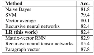
Stanford sentiment treebank (Socher et al., 2013)—Table 2. A sentence-level sentiment analysis dataset of rottentomatoes.com movie re-views:http://nlp.stanford.edu/sentiment. We use the

binary classification task where the goal is to pre-dict whether a review is positive or negative (no neutral). Our logistic regression model outperforms the baseline SVM reported by Socher et al. (2013), who used only unigrams but did not specify the weighting scheme for their SVM baseline. While our result is still below the state-of-the-art based on the the recursive neural tensor networks (Socher et al., 2013) and the paragraph vector (Le and Mikolov, 2014), we show that logistic regression is comparable with recursive and matrix-vector neu-ral networks (Socher et al., 2011; Socher et al., 2012).

Method Acc.

Na¨ıve Bayes 81.8

SVM 79.4

Vector average 80.1

Recursive neural networks 82.4

LR (this work) 82.4

Matrix-vector RNN 82.9

Recursive neural tensor networks 85.4

Paragraph vector 87.8

Table 2: Comparisons on the Stanford sentiment treebank dataset. Scores are as reported by Socher et al. (2013) and Le and Mikolov (2014). Test size= 6,920.

Amazon electronics (McAuley and Leskovec, 2013)—Table 3. A binary sentiment analy-sis dataset of Amazon electronics product re-views:http://riejohnson.com/cnn data.html. The

best-performing methods on this dataset are based on convolutional neural networks (Johnson and Zhang, 2015).4 _{Our method is on par with the}

second-best of these, outperforming all of the reported feed-forward neural networks and SVM variants Johnson and Zhang used as baselines. They varied

the representations, and used log term frequency and normalization to unit vectors as the weighting scheme, after finding that this outperformed term frequency. Our method achieved the best perfor-mance with binary weighting, which they did not consider.

IMDB movie reviews (Maas et al., 2011)— Table 3. A binary sentiment analysis dataset of highly polar IMDB movie reviews:

http://ai.stanford.edu/~amaas/data/sentiment. The

results parallel those for Amazon electronics; our method comes close to convolutional neural networks (Johnson and Zhang, 2015), which are state-of-the-art.5 _{It outperforms SVMs and}

feed-forward neural networks, the restricted Boltzmann machine approach presented by Dahl et al. (2012), and compressive feature learning (Paskov et al., 2013).6

Method _AmazonAccuracy_IMDB

SVM-unigrams 88.29 88.64

RBM 89.23

SVM-{1,2}-grams 90.95 90.26 Compressive feature learning 90.40 SVM-{1,2,3}-grams 91.29 90.58 LR-{1,2,3,4,5}-grams 90.60 NN-{1,2,3}-grams 91.52 90.83

LR (this work) 91.56 90.85

Bag of words CNN 91.61 91.34

Sequential CNN 92.52 91.61

Table 3: Comparisons on the Amazon electronics and IMDB reviews datasets. SVM results are from Wang and Manning (2012), the RBM (restricted Bolzmann machine) result is from Dahl et al. (2012), NN and CNN results are from Johnson and Zhang (2015), and LR-{1,2,3,4,5}-grams and compres-sive feature learning results are from Paskov et al. (2013). Test size= 20,000for both datasets.

Congressional vote (Thomas et al., 2006)—Table 4. A dataset of transcripts from the U.S. Congressional debates:

http://www.cs.cornell.edu/~ainur/sle-data.html. Similar

to previous work (Thomas et al., 2006; Bansal et al., 2008; Yessenalina et al., 2010), we consider the task to predict the vote (“yea” or “nay”) for the speaker of each speech segment (speaker-based speech-segment classification). Our method outperforms the best results of Yessenalina et al. (2010), which use a multi-level structured

5_{As noted, semi-supervised and ensemble methods are} excluded for a fair comparison.

6_{This approach is based on minimum description length,} using unlabeled data to select a set of higher-ordern-grams to use as features.

model based on a latent-variable SVM. We show comparisons to two weaker baselines as well.

Method Acc.

SVM-link 71.28

Min-cut 75.00

SVM-SLE 77.67

LR (this work) 78.59

Table 4: Comparisons on the congress vote dataset. SVM-link exploits SVM-link structures (Thomas et al., 2006); the min-cut result is from Bansal et al. (2008); and SVM-SLE result is reported by Yessenalina et al. (2010). Test size= 1,175.

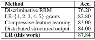
20 Newsgroups (Lang, 1995) all topics—Table 6. 20 Newsgroups is a benchmark topic classifica-tion dataset:http://qwone.com/~jason/20Newsgroups. There are 20 topics in this dataset. Our method outperforms state-of-the-art methods including the distributed structured output model (Srikumar and Manning, 2014).7 _{The strong logistic regression}

baseline from Paskov et al. (2013) uses all 5-grams, heuristic normalization, and elastic net regulariza-tion; our method found that unigrams and bigrams, with binary weighting and`2penalty, achieved far

better results.

Method Acc.

Discriminative RBM 76.20 LR-{1,2,3,4,5}-grams 82.80 Compressive feature learning 83.00 Distributed structured output 84.00

LR (this work) 87.84

Table 6: Comparisons on the 20 Newsgroups dataset for classifying documents into all topics. The disriminative RBM result is from Larochelle and Bengio (2008); compressive feature learning and LR-5-grams results are from Paskov et al. (2013), and the distributed structured output result is from Srikumar and Manning (2014). Test size= 9,052.

20 Newsgroups: talk.religion.miscvs.alt.atheism

andcomp.graphicsvs.comp.windows.x. We

de-rived three additional topic classification tasks from the 20N dataset. The first and second tasks are

talk.religion.miscvs.alt.atheism(test size= 686) and

comp.graphicsvs.comp.windows.x(test size= 942).

Wang and Manning (2012) report a bigram na¨ıve Bayes model achieving 85.1% and 91.2% on these tasks, respectively (best single model results).8 _Our

7_{This method was designed for structured prediction, but} Srikumar and Manning (2014) also applied it to classification. It attempts to learn a distributed representation for features and for labels. The authors used unigrams and did not discuss the weighting scheme.

Dataset Acc. nmin nmax Weighting Stopword removal? Reg. Strength Conv.

Stanford sentiment 82.43 1 2 tf-idf F `2 10 0.098

Amazon electronics 91.56 1 3 binary F `2 120 0.022

IMDB reviews 90.85 1 2 binary F `2 147 0.019

Congress vote 78.59 2 2 binary F `2 121 0.012

20N all topics 87.84 1 2 binary F `2 16 0.008

20N all science 95.82 1 2 binary F `2 142 0.007

20N atheist/religion 86.32 1 2 binary T `1 41 0.011

20N x/graphics 92.09 1 1 binary T `2 91 0.014

Table 5: Classification accuracies and the best hyperparameters for each of the datasets in our experiments. “Acc” shows accuracies for our logistic regression model. “Min” and “Max” correspond to the minn-grams and maxn-grams respectively. “Reg.” is the regularization type, “Strength” is the regularization strength, and “Conv.” is the convergence tolerance. For

regularization strength, we round it to the nearest integer for readability.

method achieves 86.3% and 92.1% using slightly different representations (see Table 5). The last task is to classify related science documents into four science topics (sci.crypt, sci.electronics, sci.space,

sci.med; test size = 1,899). We were not able to

find previous results that are comparable to ours on this task; we include our result (95.82%) to enable further comparisons in the future.

5 Discussion

Optimized representations. For each task, the chosen representation is different. Out of all possi-ble choices in our experiments (Tapossi-ble 1), each of them is used by at least one of the datsets (Table 5). For example, on the Congress vote dataset, we only need to use bigrams, whereas on the Amazon elec-tronics dataset we need to use{1,2,3}-grams. The binary weighting scheme works well for most of the datasets, except the sentence-level sentiment analysis task, where the tf-idf weighting scheme was selected. `2regularization was best in all cases

but one. We do not believe that an NLP expert would be likely to make these particular choices, except through the same kind of trial-and-error pro-cess our method automates efficiently.

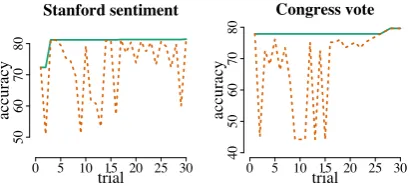
Number of trials. We ran 30 trials for each dataset in our experiments. Figure 1 shows each trial accuracy and the best accuracy on develop-ment data as we increase the number of trials for two datasets. We can see that 30 trials are gener-ally enough for the model to obtain good results, although the search space is large.

Transfer learning and multitask setting. We treat each dataset independently and create a sep-arate model for each of them. It is also possible to learn from previous datasets (i.e., transfer learn-ing) or to learn from all datasets simultaneously (i.e., multitask learning) to improve performance. This has the potential to reduce the number of trials

Stanford sentiment

trial

ac

cura

cy

0 5 10 15 20 25 30

50

60

70

80

Congress vote

trial

ac

cura

cy

0 5 10 15 20 25 30

40

50

60

70

80

Figure 1: Classification accuracies on development data for Stanford sentiment treebank (left) and congressional vote (right) datasets. In each plot, the green solid line indicates the best accuracy found so far, while the dotted orange line shows accuracy at each trial. We can see that in general the model is able to obtain reasonably good representation in 30 trials.

required even further. See Bardenet et al. (2013), Swersky et al. (2013), and Yogatama and Mann (2014) for more about how to perform Bayesian optimization in these settings.

Beyond supervised learning. Our framework could also be extended to unsupervised and semi-supervised models. For example, in document clus-tering (e.g.,k-means), we also need to construct representations for documents. Log-likelihood might serve as a performance function. A range of random initializations might be considered. Inves-tigation of this approach for nonconvex problems is an exciting area for future work.

6 Conclusion

We used Bayesian optimization to optimize choices about text representations for various categoriza-tion problems. Our technique identifies settings for a standard linear model (logistic regression) that are competitive with far more sophisticated meth-ods on topic classification and sentiment analysis. Acknowledgments

References

Mohit Bansal, Clair Cardie, and Lillian Lee. 2008. The power of negative thinking: Exploiting label disagreement in the min-cut classification framework. InProc. of COLING.

Remi Bardenet, Matyas Brendel, Balazs Kegl, and Michele Sebag. 2013. Collaborative hyperparam-eter tuning. InProc. of ICML.

James Bergstra, Remi Bardenet, Yoshua Bengio, and Balazs Kegl. 2011. Algorithms for hyper-parameter optimization. InNIPS.

James Bergstra, Daniel Yamins, and David Cox. 2013. Making a science of model search: Hyperparameter optimization in hundreds of dimensions for vision architectures. InProc. of ICML.

Walter Daelemans, Veronique Hoste, Fien De Meulder, and Bart Naudts. 2003. Combined optimization of feature selection and algorithm parameters in ma-chine learning of language. InProc. of ECML.

George E. Dahl, Ryan P. Adams, and Hugo Larochelle. 2012. Training restricted Boltzmann machines on word observations. InProc. of ICML.

Matthew Hoffman, Eric Brochu, and Nando de Freitas. 2011. Portfolio allocation for Bayesian optimization. InProc. of UAI.

Frank Hutter, Holger H. Hoos, and Kevin Leyton-Brown. 2011. Sequential model-based optimization for gen-eral algorithm configuration. InProc. of LION.

Rie Johnson and Tong Zhang. 2015. Effective use of word order for text categorization with convolutional neural networks. InProc. of NAACL.

Donald R. Jones. 2001. A taxonomy of global optimiza-tion methods based on response surfaces.Journal of Global Optimization, 21:345–385.

Ken Lang. 1995. Newsweeder: Learning to filter net-news. InProc. of ICML.

Hugo Larochelle and Yoshua Bengio. 2008. Classi-fication using discriminative restricted Boltzmann machines. InProc. of ICML.

Quoc V. Le and Tomas Mikolov. 2014. Distributed representations of sentences and documents. InProc. of ICML.

Omer Levy, Yoav Goldberg, and Ido Dagan. 2015. Im-proving distributional similarity with lessons learned from word embeddings. Transactions of the Associa-tion for ComputaAssocia-tional Linguistics, 3:211–225.

Andrew L. Maas, Raymond E. Daly, Peter T. Pham, Dan Huang, Andrew Y. Ng, and Christopher Potts. 2011. Learning word vectors for sentiment analysis. InProc. of ACL.

Julian McAuley and Jure Leskovec. 2013. Hidden factors and hidden topics: understanding rating di-mensions with review text. InProc. of RecSys. Hristo S. Paskov, Robert West, John C. Mitchell, and

Trevor J. Hastie. 2013. Compressive feature learning. InProc of NIPS.

Carl Edward Rasmussen and Christopher K. I. Williams. 2006. Gaussian Processes for Machine Learning. The MIT Press.

Jasper Snoek, Hugo Larrochelle, and Ryan P. Adams. 2012. Practical Bayesian optimization of machine learning algorithms. InNIPS.

Richard Socher, Jeffrey Pennington, Eric H. Huang, Andrew Y. Ng, and Christopher D. Manning. 2011. Semi-supervised recursive autoencoders for predict-ing sentiment distributions. InProc. of EMNLP. Richard Socher, Brody Huval, Christopher D. Manning,

and Andrew Y. Ng. 2012. Semantic compositionality through recursive matrix-vector spaces. InProc. of EMNLP.

Richard Socher, Alex Perelygin, Jean Wu, Jason Chuang, Chris Manning, Andrew Ng, and Chris Potts. 2013. Recursive deep models for semantic compo-sitionality over a sentiment treebank. In Proc. of EMNLP.

Vivek Srikumar and Christopher D. Manning. 2014. Learning distributed representations for structured output prediction. InNIPS.

Niranjan Srinivas, Andreas Krause, Sham Kakade, and Matthias Seeger. 2010. Gaussian process optimiza-tion in the bandit setting: No regret and experimental design. InProc. of ICML.

Kevin Swersky, Jasper Snoek, and Ryan P. Adams. 2013. Multi-task Bayesian optimization. InNIPS. Matt Thomas, Bo Pang, and Lilian Lee. 2006. Get out

the vote: Determining support or opposition from congressional floor-debate transcripts. In Proc. of EMNLP.

Julien Villemonteix, Emmanuel Vazquez, and Eric Walter. 2009. An informational approach to the global optimization of expensive-to-evaluate func-tions. Journal of Global Optimization, 44(4):509– 534.

Sida Wang and Christopher D. Manning. 2012. Base-lines and bigrams: Simple, good sentiment and topic classification. InProc. of ACL.

Ainur Yessenalina, Yisong Yue, and Claire Cardie. 2010. Multi-level structured models for document sentiment classification. InProc. of EMNLP. Dani Yogatama and Gideon Mann. 2014. Efficient