58
Layerwise Relevance Visualization in Convolutional Text Graph
Classifiers
Robert Schwarzenberg, Marc H ¨ubner, David Harbecke, Christoph Alt, Leonhard Hennig
German Research Center for Artificial Intelligence (DFKI), Berlin, Germany
Abstract
Representations in the hidden layers of Deep Neural Networks (DNN) are often hard to in-terpret since it is difficult to project them into an interpretable domain. Graph Convolutional Networks (GCN) allow this projection, but ex-isting explainability methods do not exploit this fact, i.e. do not focus their explanations on intermediate states. In this work, we present a novel method that traces and visualizes fea-tures that contribute to a classification decision in the visible and hidden layers of a GCN. Our method exposes hidden cross-layer dynamics in the input graph structure. We experimen-tally demonstrate that it yields meaningful lay-erwise explanations for a GCN sentence clas-sifier.
1 Introduction
A Deep Neural Network (DNN) that offers – or from which we can retrieve – explanations for its decisions arguably is easier to improve and de-bug than a black box model. Loosely following Montavon et al. (2018), we understand an expla-nation as a “collection of features (...) that have contributed for a given example to produce a deci-sion.” For humans to make sense of an explanation it needs to be expressed in a human-interpretable domain, which is often the input space (Montavon et al.,2018).
For instance, in the vision domain Bach et al. (2015) propose the Layerwise Relevance Propa-gation (LRP) algorithm that propagates contribu-tions from an output activation back to the first layer, the input pixel space. Arras et al. (2017) implement a similar strategy for NLP tasks, where contributions are propagated into the word vector space and then summed up over the word vector dimensions to create heatmaps in the plain text in-put space.
In the course of the backpropagation of con-tributions, hidden layers in the DNN are visited, but rarely inspected.1 A major challenge when in-specting and interpreting hidden states lies in the fact that a projection into an interpretable domain is often made difficult by the linearity, non-locality and dimension reduction/expansion across hidden layers.
In this work, we present an explainability method that visits and projects visible and hidden states in Graph Convolutional Networks (GCN) (Kipf and Welling,2016) onto the interpretable in-put space. Each GCN layer fuses neighborhoods in the input graph. For this fusion to work, GCNs need to replicate the input adjacency at each layer. This allows us to project their intermediate repre-sentations back onto the graph.
Our method, layerwise relevance visualization (LRV), not only visualizes static explanations in the hidden layers, but also tracks and visual-izes hidden cross-layer dynamics, as illustrated in Fig. 1. In a qualitative and a quantitative anal-ysis, we experimentally demonstrate that our ap-proach yields meaningful explanations for a GCN sentence classifier.
2 Methods
In this section we explain how we combine GCNs and LRP for layerwise relevance visualization. We begin with a short recap of GCNs and LRP to es-tablish a basis for our approach and to introduce notation.
2.1 Graph Convolutional Networks
Assume a graph G represented by ( ˜A, H(0))
whereA˜is a degree-normalized adjacency matrix, which introduces self loops to the nodes inG, and
A total of 116 patients were randomized . (2.08) (14.21) (8.56) (41.18) (0.0) (30.28) (2.56) (1.12)
det
nmod case
nummod nsubjpass
auxpass punct
GCN GCN FC
A total of 116 patients were randomized . (1.36) (6.29) (4.58) (25.71) (19.46) (22.41) (19.13) (1.07)
det
nmod case
nummod nsubjpass
auxpass punct
GCN GCN FC
A total of 116 patients were randomized . (0.74) (12.64) (1.15) (18.41) (20.87) (17.91) (27.39) (0.9)
det
nmod case
nummod nsubjpass
auxpass punct
[image:2.595.124.480.60.321.2]GCN GCN FC
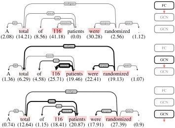
Figure 1: Layerwise Relevance Visualization in a Graph Convolutional Network. Left: Projection of relevance percentages (in brackets) onto the input graph structure (red highlighting). Edge strength is proportional to the relevance percentage an edge carried from one layer to the next. Right: Architecture (replicated at each layer) of the GCN sentence classifier (input bottom, output top). Node and edge relevance were normalized layerwise. The predicted label of the input wasRESULT, as was the true label.
H(0)∈IRn×dan embedding matrix of thennodes inG, ordered in compliance withA. A GCN layer˜ propagates such graph inputs according to
H(l+1)=σ
˜
AH(l)W(l)
, (1)
which can be decomposed into a feature projec-tion H0(l) = H(l)W(l) and an adjacency projec-tionAH˜ 0(l), followed by a non-linearityσ.
The adjacency projection fuses each node with the features in its effective neighborhood. At each GCN layer, the effective neighborhood becomes one hop larger, starting with a one-hop neighbor-hood in the first layer. The last layer in a GCN classifier typically is fully connected (FC) and projects its inputs onto class probabilities.
2.2 Layerwise Relevance Propagation
To receive explanations for the classifications of a GCN classifier, we apply LRP. LRP explains a neuron’s activation by computing how much each of its input neurons contributed2to the activation. Contributions are propagated back layerwise.
2
We use the terms contribution and relevance inter-changeably.
Montavon et al. (2017) show that the positive contribution of neuron h(il), as defined in Bach et al.(2015) with thez+-rule, is equivalent to
Ri =X
j
h(il)w+ij
P kh
(l)
k w
+
kj
Rj, (2)
where P
k sums over the neurons in layerl and P
j over the neurons in layer (l + 1). Eq. 2 only allows positive inputs, which each layer re-ceives if the previous layers are activated using ReLUs.3 LRP has an important property, namely the relevance conservation property: P
jRj←k = Rk, Rj = PkRj←k, which not only conserves
relevance from neuron to neuron but also from layer to layer (Bach et al.,2015).
2.3 Layerwise Relevance Visualization
We combine graph convolutional networks and layerwise relevance propagation for layerwise rel-evance visualization as follows. During train-ing, GCNs receive input graphs in the form of
( ˜A, H(0)) tuples. This is efficient and allows
3
batching but it poses a problem for LRP: If the adjacency matrix is considered part of the input, one could argue that it should receive relevance mass. This, however, would make it hard to meet the conservation property.
Instead, we treat A˜ as part of the model in a post-hoc explanation phase, in which we construct an FC layer withA˜as its weights. The GCN layer then consists of two FC sublayers. During the for-ward pass, the first one performs the feature pro-jection and the second one – the newly constructed one – the adjacency projection.
To make use of Eq. 2 in the adjacency layer, we need to avoid propagating negative activations. This is why we apply the ReLU activation early, right after the feature projection, which yields the propagation rule
H(l+1) = ˜Aσ(H(l)W(l)). (3)
When unrolled, this effectively just moves one ad-jacency projection from inside the first ReLU to outside the last ReLU. Alternatively, it should be possible to first perform the adjacency projection and afterwards the feature projection.
Eq. 3 allows us to directly apply Eq. 2 to the two projection sublayers in a GCN layer. Dur-ing LRP, we cache the intermediate contribution maps R(l) ∈ IRn×f that we receive right after we propagated past the feature projection sublayer and compute nodei’s contribution in that layer as R(i(l)) = P
cR
(l)
ic. In addition, we also compute the edge relevancee((li,j))between nodesiandjas the amount of relevance that it carried from layer l−1to layerl.
In what follows, we useR(i(l))ande(ijl)to visu-alize hidden state dynamics (i.e. relevance flow) in the input graph. Furthermore, similar to Xie and Lu (2019), we make use of perturbation experi-ments to verify that our method indeed identifies the relevant components in the input graph.
3 Experiments
Our experiments are publicly available: https://github.com/DFKI-NLP/lrv/. We trained a GCN sentence classifier on a 20k subset of the PubMed 200k RCT dataset ( Der-noncourt and Lee, 2017). The dataset contains scientific abstracts in which each sentence is annotated with either of the 5 labels BACK-GROUND, OBJECTIVE, METHOD, RESULT, or CONCLUSION. Dernoncourt and Lee (2017)
describe the task as a sequential classification task since all sentences in one abstract are classified in sequence, but we treat it as a conventional sentence classification task, classifying each sentence in isolation.
In a preprocessing step, we used ScispaCy (Neumann et al., 2019) for tokenization and de-pendency parsing to generate the input graphs for the GCN sentence classifier. For the node em-beddings in the dependency graph, we utilized pre-trained fastText embeddings (Mikolov et al., 2018). Edge type information was discarded.
Our classifier, implemented and trained using PyTorch (Paszke et al., 2017), consists of two stacked GCN layers (Eq.3), followed by a max-pooling operation and a subsequent FC layer. All layers were trained without bias and optimized with the Adam optimizer (Kingma and Ba,2014). After each optimization step we clamped the neg-ative weights of the last FC layer to avoid negneg-ative outputs.
During training, we batched inputs, but in the post-hoc explanation phase, single graphs from the test set were forwarded through the network to im-plement the strategy outlined in Sec.2.3. We first constructed the adjacency layer withA, then per-˜ formed a forward pass during which we cached the inputs at each layer for LRP.
LRP started at the output neuron with the max-imal activation, before the softmax normalization. For all intermediate layers we used Eq.2. Since coefficients in the input word vectors are nega-tive, we used a special propagation rule (Montavon et al., 2017), which we omit here, due to space contraints. We cached the intermediate contribu-tion maps right after the max-pooling operacontribu-tion, after the second and after the first (input space) feature projection layers in the GCN layers.
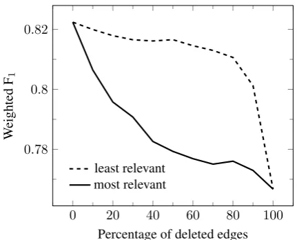
For the qualitative analysis, we visualized the contributions of each node at each layer as well as the relevance flow over the graph’s edges across layers, as outlined in Sec.2.3. For the quantita-tive validation, we deleted a growing portion of the globally most relevant edges (starting with the most relevant ones) and monitored the model’s classification performance. In a second experi-ment, we did the same starting with the least rele-vant edges. Here,global edge relevancerefers to the sum of an edge’s relevance across all layers, P
le
(l)
4 Results
After training, our model achieved a weighted F1
score of 0.822 on the official (20k) test set. We then performed the post-hoc explanation with the trained model, receiving layerwise explanations as the one depicted in Fig.1. More examples can be found in the appendix.
Fig. 1 (top) shows which vectors in the final layer the GCN bases its classification decision on. The middle and bottom segments reveal how much relevant information the model fused in these vec-tors from neighboring nodes during the forward pass:
According to the LRV in Fig. 1, the model primarily bases its classification decision on the fusion of the vector representations of total,
patients, and116. The vector representations of these nodes are accumulated in the vector of
116in two steps.
Interestingly, the vector of patients con-tributes a larger portion after it has been fused with
total. Furthermore, randomized becomes more relevant after the first GCN layer, contribut-ing to the second most relevant n-gram(were, randomized). Other n-grams, such as (A, total)or(of, patients)appear less rele-vant.
Note that if we had simply redistributed the contributions in the final layer, using only the adjacency matrix, without considering the acti-vations in the forward pass as LRP does, these n-grams would have received an unsubstantiated share. Furthermore, a conventional, single expla-nation in the input space would have hardly re-vealed the hidden dynamics discussed above.
As explained in Sec. 3, we also conducted in-put perturbation experiments to validate that our method indeed identifies the graph components that are relevant to the GCN decision. Fig.2 sum-marizes the results: The performance of our model degrades much faster when we delete edges that contributed a lot to the model’s decision, accord-ing to our method. We take this as evidence that our method indeed correctly identifies the relevant components in the input graphs.
5 Related Work
Niepert et al. (2016); Wu et al. (2019) introduce graph networks that natively support feature visu-alization (explanations) but their models are not
0 20 40 60 80 100
0.78 0.8 0.82
Percentage of deleted edges
W
eighted
F1
least relevant most relevant
Figure 2: Perturbation experiment.
graph convolutional networks in the sense ofKipf and Welling(2016) that we address here.
Veliˇckovi´c et al. (2017) propose Graph Atten-tion Networks and also project an explanaAtten-tion of a hidden representation onto the input graph. They do not, however, continue across multiple layers. Furthermore, their explanation technique differs from ours. The authors use attention coefficients to scale edge thicknesses in their explanatory visu-alization. In contrast, we base edge relevance on the amount of relevance an edge carried from one layer to the next, according to LRP. Our method does this in a conventional GCN, which does not apply the attention mechanism.
The body of work on the explainability of graph neural nets also includes the GNN explainer by Ying et al.(2019), a model-agnostic explainabil-ity method. Since their method is model-agnostic, it can be applied to GCNs. Nevertheless, it would not reveal hidden dynamics, as our method does.
[image:4.595.308.524.59.233.2]our approach, suggest to trace (and visualize) ex-planations over feature-less edges. Both works, however, address a different task from ours: In contrast to our graph classification task, they per-form node classification and identify k-hop neigh-bor contributions in the proximity of a central node of interest.
6 Conclusions
We presented layerwise relevance visualization in convolutional text graph classifiers. We demon-strated that our approach allows to track, visualize and inspect visible as well as hidden state dynam-ics. We conducted qualitative and quantitative ex-periments to validate the proposed method.
This is a focused contribution; further research should be conducted to test the approach in other domains and on other data sets. Future versions should also exploit LRP’s ability to expose nega-tive evidence and the method could be extended to node classifiers.
7 Acknowledgements
This research was partially supported by the Ger-man Federal Ministry of Education and Research through the project DEEPLEE (01IW17001). We would also like to thank the anonymous reviewers for their feedback on the paper and Arne Binder for his feedback on the code base.
References
Leila Arras, Franziska Horn, Gr´egoire Montavon, Klaus-Robert M¨uller, and Wojciech Samek. 2017. ”What is relevant in a text document?”: An in-terpretable machine learning approach. PloS one, 12(8):e0181142.
Sebastian Bach, Alexander Binder, Gr´egoire Mon-tavon, Frederick Klauschen, Klaus-Robert M¨uller, and Wojciech Samek. 2015. On pixel-wise explana-tions for non-linear classifier decisions by layer-wise relevance propagation. PLoS ONE, 10(7):e0130140.
Federico Baldassarre and Hossein Azizpour. 2019. Ex-plainability techniques for graph convolutional net-works. arXiv preprint arXiv:1905.13686.
Franck Dernoncourt and Ji Young Lee. 2017. Pubmed 200k rct: a dataset for sequential sentence classifica-tion in medical abstracts. IJCNLP 2017, page 308.
Diederik P Kingma and Jimmy Ba. 2014. Adam: A method for stochastic optimization. arXiv preprint arXiv:1412.6980.
Thomas N Kipf and Max Welling. 2016. Semi-supervised classification with graph convolutional networks. arXiv preprint arXiv:1609.02907.
Tomas Mikolov, Edouard Grave, Piotr Bojanowski, Christian Puhrsch, and Armand Joulin. 2018. Ad-vances in pre-training distributed word representa-tions. InProceedings of the International Confer-ence on Language Resources and Evaluation (LREC 2018).
Gr´egoire Montavon, Sebastian Lapuschkin, Alexander Binder, Wojciech Samek, and Klaus-Robert M¨uller. 2017. Explaining nonlinear classification decisions with deep taylor decomposition. Pattern Recogni-tion, 65:211–222.
Gr´egoire Montavon, Wojciech Samek, and Klaus-Robert M¨uller. 2018. Methods for interpreting and understanding deep neural networks. Digital Signal Processing, 73:1–15.
Mark Neumann, Daniel King, Iz Beltagy, and Waleed Ammar. 2019. Scispacy: Fast and robust models for biomedical natural language processing.
Mathias Niepert, Mohamed Ahmed, and Konstantin Kutzkov. 2016. Learning convolutional neural net-works for graphs. In International conference on machine learning, pages 2014–2023.
Adam Paszke, Sam Gross, Soumith Chintala, Gre-gory Chanan, Edward Yang, Zachary DeVito, Zem-ing Lin, Alban Desmaison, Luca Antiga, and Adam Lerer. 2017. Automatic differentiation in pytorch.
Phillip E Pope, Soheil Kolouri, Mohammad Rostami, Charles E Martin, and Heiko Hoffmann. 2019. Ex-plainability methods for graph convolutional neural networks. InProceedings of the IEEE Conference on Computer Vision and Pattern Recognition, pages 10772–10781.
Petar Veliˇckovi´c, Guillem Cucurull, Arantxa Casanova, Adriana Romero, Pietro Lio, and Yoshua Bengio. 2017. Graph attention networks. arXiv preprint arXiv:1710.10903.
Felix Wu, Tianyi Zhan, Amauri Holonda de Souza Jr., Christopher Fifty, Tao Yu, and Kilian Weinberger Q. 2019. Simplifying graph convolutional network. arXiv preprint.
Shangsheng Xie and Mingming Lu. 2019. Interpret-ing and understandInterpret-ing graph convolutional neural network using gradient-based attribution methods. arXiv preprint arXiv:1903.03768.